Take-home Exercise 2: Applied Spatial Interaction Models - A case study of Singapore public bus commuter flows

1 Overview

Urban mobility, characterized by the daily commute of urban dwellers from homes to workplaces, presents complex challenges for transport operators and urban managers. Traditional approaches to understanding these mobility patterns, such as commuter surveys, are often hindered by high costs, time-consuming processes, and the rapid obsolescence of collected data. However, the digitalization of city-wide urban infrastructures, including public buses, mass rapid transits, and other utilities, alongside the advent of pervasive computing technologies like GPS and SMART cards, offers a new paradigm in tracking and analyzing urban movement.

Objectives

Aim

This assignment is driven by two primary motivations. First, despite the growing availability of open data for public use, there is a noticeable gap in applied research demonstrating how these diverse data sources can be effectively integrated and analyzed to inform policy-making decisions. Second, there is a need to showcase how GDSA can be utilized in practical decision-making scenarios.

The core task of this assignment is to conduct a case study that exhibits the potential value of GDSA. By leveraging publicly available data from multiple sources, the goal is to build spatial interaction models that unravel the factors influencing urban mobility patterns, particularly focusing on public bus transit. This exercise aims to bridge the gap between the abundance of geospatially-referenced data and its practical application, thereby enhancing the return on investment in data collection and management, and ultimately supporting informed policy-making in urban mobility.

Tasks

The specific tasks of this take-home exercise are as follows:

Geospatial Data Science

• Derive an analytical hexagon data of 375m (this distance is the perpendicular distance between the centre of the hexagon and its edges) to represent the traffic analysis zone (TAZ).

• With reference to the time intervals provided in the table below, construct an O-D matrix of commuter flows for a time interval of your choice by integrating Passenger Volume by Origin Destination Bus Stops and Bus Stop Location from LTA DataMall. The O-D matrix must be aggregated at the analytics hexagon level

  Peak hour period	Bus tap on time
  Weekday morning peak	6am to 9am
  Weekday afternoon peak	5pm to 8pm
  Weekend/holiday morning peak	11am to 2pm
  Weekend/holiday evening peak	4pm to 7pm

• Display the O-D flows of the passenger trips by using appropriate geovisualisation methods (not more than 5 maps).

• Describe the spatial patterns revealed by the geovisualisation (not more than 100 words per visual).

• Assemble at least three propulsive and three attractiveness variables by using aspatial and geospatial from publicly available sources.

• Compute a distance matrix by using the analytical hexagon data derived earlier.

Spatial Interaction Modelling

• Calibrate spatial interactive models to determine factors affecting urban commuting flows at the selected time interval.

• Present the modelling results by using appropriate geovisualisation and graphical visualisation methods. (Not more than 5 visuals)

• With reference to the Spatial Interaction Model output tables, maps and data visualisation prepared, describe the modelling results. (not more than 100 words per visual).

2 Loading Packages

Packages

The following packages will be used for this exercise:

Package	Description
tmap	For thematic mapping
sf & sp	For importing, integrating, processing, and transforming geospatial data
tidyverse	For non-spatial data wrangling
DT	For creating and working with html tables
performance	For computing model comparison metrics
reshape2	For data transformation between wide and long formats
ggpubr and gtsummary	For creating publication quality analytical and summary tables
stplanr	For transport planning and analysis
knitr	For dynamic report generation
scales	For scaling graphs
corrplot	For visualising correlation matrix
plotly	For interactive and dynamic plots

Code

The code chunk below, using p_load function of the pacman package, ensures that packages required are installed and loaded in R.

pacman::p_load(tmap, sf, sp, 
               tidyverse, DT, performance, 
               reshape2, ggpubr, stplanr,
               knitr, scales, corrplot, 
               gtsummary, plotly)

3 Data Preparation

For the purpose of this assignment, the following data will be used:

	Type	Name	As of Date	Format	Source
1	Aspatial	Passenger Volume by Origin Destination Bus Stops	Oct 2023	.csv	LTA DataMall
2	Aspatial	School Directory and Information (General information of schools)	Mar 2022	.csv	Data.gov.sg
3	Aspatial	HDB Property Information (Geocoded)	Sep 2021	.csv	Courtesy of Prof T. S. Kam
4	Geospatial	Bus Stop Location	Jul 2023	.shp	LTA DataMall
5	Geospatial	Train Station Exit Point	Aug 2023	.shp	LTA DataMall
6	Geospatial	Master Plan 2019 Subzone Boundary	2019	.shp	Courtesy of Prof T.S. Kam
7	Geospatial	Business (incl. industrial parks), FinServ, Leisure&Recreation and Retails (Geospatial data sets of the locations of business establishments, entertainments, food and beverage outlets, financial centres, leisure and recreation centres, retail and services stores/outlets compiled for urban mobility study)		.shp	Courtesy of Prof T.S. Kam

3.1 O-D Data

Importing csv

Passenger Volume by Origin Destination Bus Stops dataset for October 2023, downloaded from LTA DataMall by using read_csv() or readr package.

odbus <- read_csv("data/aspatial/origin_destination_bus_202310.csv")

Attributes

glimpse() of the dplyr package allows us to see all columns and their data type in the data frame.

glimpse(odbus)

Rows: 5,694,297
Columns: 7
$ YEAR_MONTH          <chr> "2023-10", "2023-10", "2023-10", "2023-10", "2023-…
$ DAY_TYPE            <chr> "WEEKENDS/HOLIDAY", "WEEKDAY", "WEEKENDS/HOLIDAY",…
$ TIME_PER_HOUR       <dbl> 16, 16, 14, 14, 17, 17, 17, 7, 14, 14, 10, 20, 20,…
$ PT_TYPE             <chr> "BUS", "BUS", "BUS", "BUS", "BUS", "BUS", "BUS", "…
$ ORIGIN_PT_CODE      <chr> "04168", "04168", "80119", "80119", "44069", "2028…
$ DESTINATION_PT_CODE <chr> "10051", "10051", "90079", "90079", "17229", "2014…
$ TOTAL_TRIPS         <dbl> 3, 5, 3, 5, 4, 1, 24, 2, 1, 7, 3, 2, 5, 1, 1, 1, 1…

Observations:

• There are 7 variables in the odbus tibble data, they are:
  • YEAR_MONTH: Month in which data is collected
  • DAY_TYPE: Weekdays or weekends/holidays
  • TIME_PER_HOUR: Hour which the passenger trip is based on, in intervals from 0 to 23 hours
  • PT_TYPE: Type of public transport, i.e. bus
  • ORIGIN_PT_CODE: Origin bus stop ID
  • DESTINATION_PT_CODE: Destination bus stop ID
• TOTAL_TRIPS: Number of trips We also note that values in ORIGIN_PT_CODE and DESTINATON_PT_CODE are in numeric data type. These should be in factor data type for further processing and georeferencing.

as.factor() can be used to convert the variables ORIGIN_PT_CODE and DESTINATON_PT_CODE from numeric to categorical data type. We use glimpse() again to check the results.

odbus$ORIGIN_PT_CODE <- as.factor(odbus$ORIGIN_PT_CODE)
odbus$DESTINATION_PT_CODE <- as.factor(odbus$DESTINATION_PT_CODE)

glimpse(odbus)

Rows: 5,694,297
Columns: 7
$ YEAR_MONTH          <chr> "2023-10", "2023-10", "2023-10", "2023-10", "2023-…
$ DAY_TYPE            <chr> "WEEKENDS/HOLIDAY", "WEEKDAY", "WEEKENDS/HOLIDAY",…
$ TIME_PER_HOUR       <dbl> 16, 16, 14, 14, 17, 17, 17, 7, 14, 14, 10, 20, 20,…
$ PT_TYPE             <chr> "BUS", "BUS", "BUS", "BUS", "BUS", "BUS", "BUS", "…
$ ORIGIN_PT_CODE      <fct> 04168, 04168, 80119, 80119, 44069, 20281, 20281, 1…
$ DESTINATION_PT_CODE <fct> 10051, 10051, 90079, 90079, 17229, 20141, 20141, 1…
$ TOTAL_TRIPS         <dbl> 3, 5, 3, 5, 4, 1, 24, 2, 1, 7, 3, 2, 5, 1, 1, 1, 1…

Note that both of them are in factor data type now.

Extracting Study Data

In our study, we would like to analyse the 1 of the peak hour periods identified. We will be analysing the Weekday Morning peak periods thereafter. Therefore, we can employ a combination of the following functions to obtain the relevant data:

Summary of the functions used as follow:

• filter(): Retains rows that satisfies our condition (i.e. Weekday Morning peak period)

• select() of dplyr package: Retains the desired variables for further analysis.

• group_by() and summarise(): Aggregates the total trips at each combination of origin bus stop, destination bus stop, and peak period.

WDMpeak <- odbus %>%
  filter(DAY_TYPE=="WEEKDAY" & (TIME_PER_HOUR >= 6 & TIME_PER_HOUR <= 9)) %>% 
  dplyr::select(5:7)  %>% 
  group_by(ORIGIN_PT_CODE, DESTINATION_PT_CODE) %>% 
  summarise(TRIPS=sum(TOTAL_TRIPS))

Let’s check the output using the glimpse() function of dplyr.

glimpse(WDMpeak)

Rows: 242,208
Columns: 3
Groups: ORIGIN_PT_CODE [5,029]
$ ORIGIN_PT_CODE      <fct> 01012, 01012, 01012, 01012, 01012, 01012, 01012, 0…
$ DESTINATION_PT_CODE <fct> 01112, 01113, 01121, 01211, 01311, 07371, 60011, 6…
$ TRIPS               <dbl> 290, 118, 77, 118, 165, 14, 30, 16, 35, 26, 2, 8, …

3.2 Geospatial Data

For the purpose of this exercise, three geospatial data will be used. They are:

• MPSZ-2019: This data provides the sub-zone boundary of URA Master Plan 2019, it helps us define the geographical boundary of Singapore.
• BusStop: This data provides the location of bus stop as at Jul 2023.
• Analytical hexagon: Hexagonal grids of 375m (this distance is the perpendicular distance between the centre of the hexagon and its edges) to represent the traffic analysis zone.

In this section, we import the shapefiles into RStudio using st_read() function of sf package. st_transform() function of sf package is used to transform the projection to coordinate reference system (CRS) 3414, which is the EPSG code for the SVY21 projection used in Singapore.

Master Plan Subzone

mpsz <- st_read(dsn="data/geospatial",                   
                layer="MPSZ-2019")%>%   
  st_transform(crs = 3414)

Reading layer `MPSZ-2019' from data source 
  `C:\kytjy\ISSS624\Take-Home_Ex\Take-Home_Ex2\data\geospatial' 
  using driver `ESRI Shapefile'
Simple feature collection with 332 features and 6 fields
Geometry type: MULTIPOLYGON
Dimension:     XY
Bounding box:  xmin: 103.6057 ymin: 1.158699 xmax: 104.0885 ymax: 1.470775
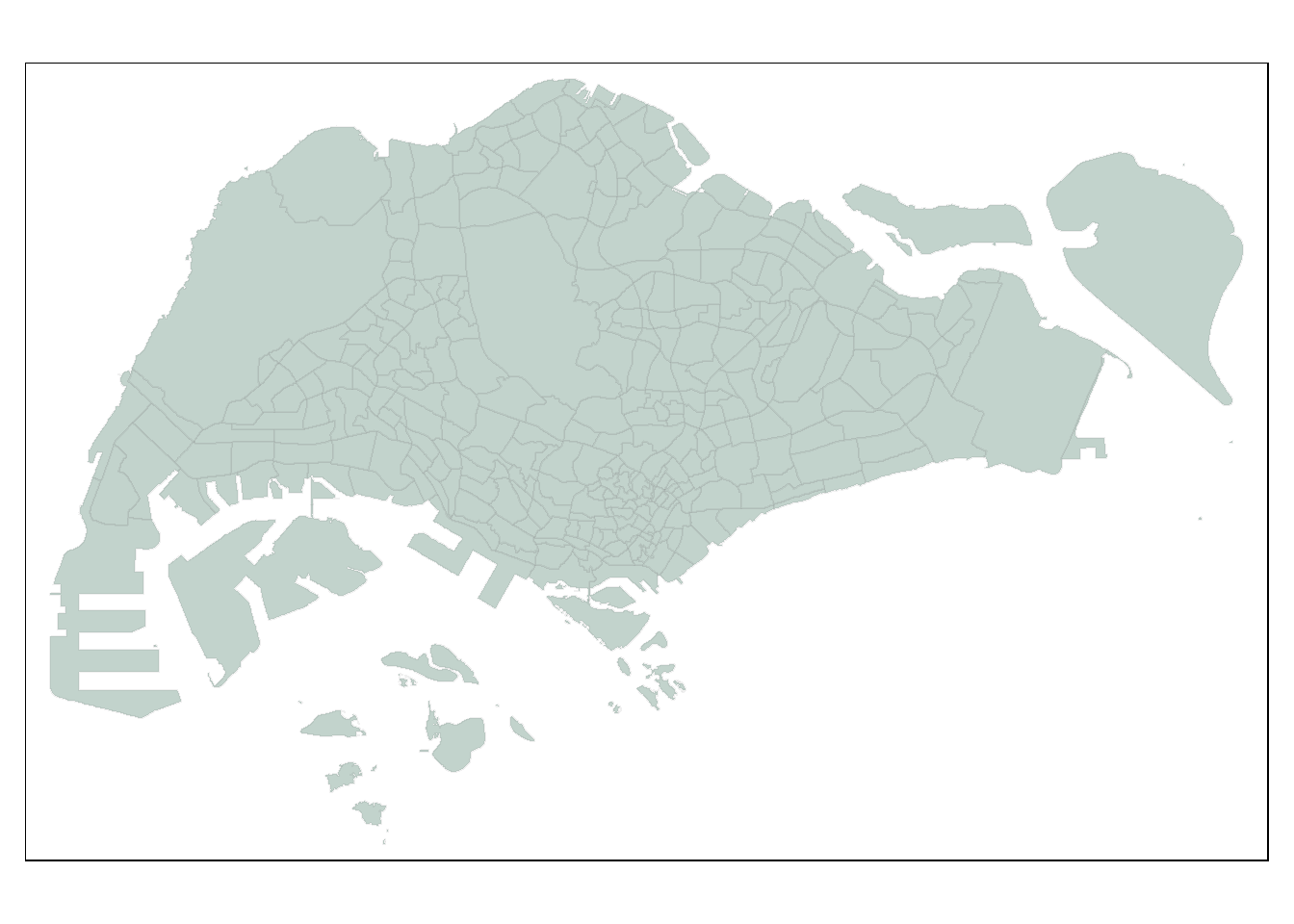
Geodetic CRS:  WGS 84

In the code chunk below, tm_shape() of tmap package is used to define the input data (i.e mpsz) and tm_polygons() is used to draw the planning subzone polygons.

Show the code

tmap_mode("plot")

tm_shape(mpsz) +
  tm_polygons(col='#C2D3CC', border.alpha = 0.1)

Bus Stop

busstop <- st_read(dsn = "data/geospatial",
                   layer = "BusStop") %>% 
  st_transform(crs = 3414)

Reading layer `BusStop' from data source 
  `C:\kytjy\ISSS624\Take-Home_Ex\Take-Home_Ex2\data\geospatial' 
  using driver `ESRI Shapefile'
Simple feature collection with 5161 features and 3 fields
Geometry type: POINT
Dimension:     XY
Bounding box:  xmin: 3970.122 ymin: 26482.1 xmax: 48284.56 ymax: 52983.82
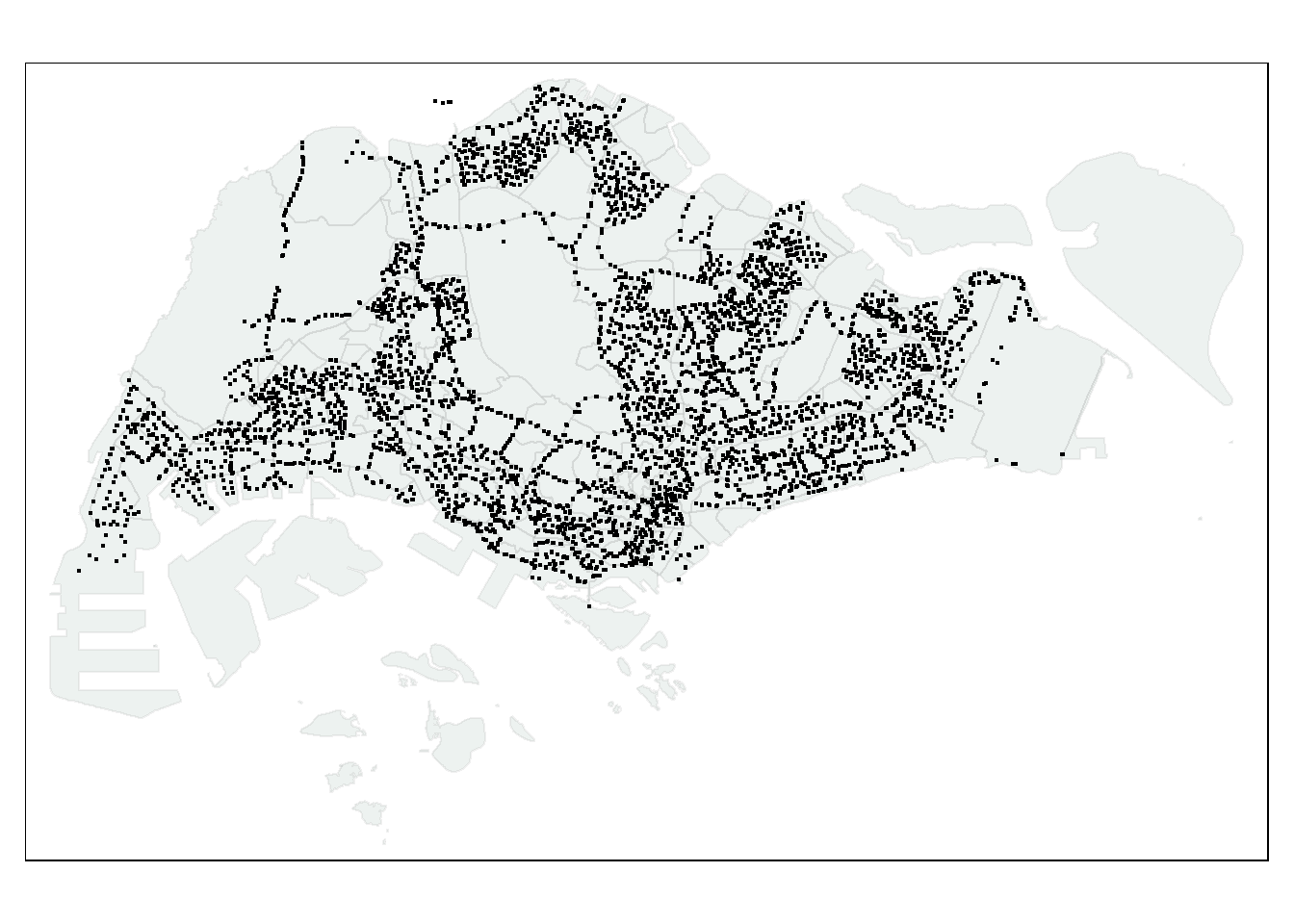
Projected CRS: SVY21

Busstop represents sf point objects for 5161 bus stop in Singapore.

To visualise the points of the bus stops, we can use tm_shape() of tmap package with each bus stop point displayed as dots. tmap_mode allows us to view static maps with plot and interactive maps with view.

Show the code

tmap_mode("plot")
tm_shape(mpsz) +
  tm_polygons(col='#C2D3CC', border.alpha = 0.1, alpha = 0.3) +
tm_shape(busstop) +
  tm_dots()+
tm_view(set.zoom.limits = c(11,14)) # to fix the map extent, so cannot zoom in too much

Before proceeding, let’s check if there are any duplicated bus stops in the dataset.

bs_dupes <- busstop %>%
  group_by(BUS_STOP_N) %>%
  filter(n() > 1) %>%
  ungroup() %>%
  arrange(BUS_STOP_N)

knitr::kable(bs_dupes)

BUS_STOP_N	BUS_ROOF_N	LOC_DESC	geometry
11009	B04	Ghim Moh Ter	POINT (23101.34 32594.17)
11009	B04-TMNL	GHIM MOH TER	POINT (23100.58 32604.36)
22501	B02	Blk 662A	POINT (13489.09 35536.4)
22501	B02	BLK 662A	POINT (13488.02 35537.88)
43709	B06	BLK 644	POINT (18963.42 36762.8)
43709	B06	BLK 644	POINT (18952.02 36751.83)
47201	UNK	NA	POINT (22616.75 47793.68)
47201	NIL	W’LANDS NTH STN	POINT (22632.92 47934)
51071	B21	MACRITCHIE RESERVOIR	POINT (28311.27 36036.92)
51071	B21	MACRITCHIE RESERVOIR	POINT (28282.54 36033.93)
52059	B03	OPP BLK 65	POINT (30770.3 34460.06)
52059	B09	BLK 219	POINT (30565.45 36133.15)
53041	B05	Upp Thomson Road	POINT (28105.8 37246.76)
53041	B07	Upp Thomson Road	POINT (27956.34 37379.29)
58031	UNK	OPP CANBERRA DR	POINT (27089.69 47570.9)
58031	UNK	OPP CANBERRA DR	POINT (27111.07 47517.77)
62251	B03	Bef Blk 471B	POINT (35500.54 39943.41)
62251	B03	BEF BLK 471B	POINT (35500.36 39943.34)
67421	B01	CHENG LIM STN EXIT B	POINT (34548.54 42052.15)
67421	NIL	CHENG LIM STN EXIT B	POINT (34741.77 42004.21)
68091	B01	AFT BAKER ST	POINT (32164.11 42695.98)
68091	B08	AFT BAKER ST	POINT (32038.84 43298.68)
68099	B02	BEF BAKER ST	POINT (32154.9 42742.82)
68099	B07	BEF BAKER ST	POINT (32004.05 43320.34)
77329	B01	BEF PASIR RIS ST 53	POINT (40765.35 39452.18)
77329	B03	Pasir Ris Central	POINT (40728.15 39438.15)
82221	B01	BLK 3A	POINT (35323.6 33257.05)
82221	B01	Blk 3A	POINT (35308.74 33335.17)
96319	NA	Yusen Logistics	POINT (42187.23 34995.78)
96319	NIL	YUSEN LOGISTICS	POINT (42187.23 34995.78)
97079	B14	OPP ST. JOHN’S CRES	POINT (44144.57 38980.25)
97079	B14	OPP ST. JOHN’S CRES	POINT (44055.75 38908.5)

The results displayed 16 pairs of duplicated BUS_STOP_N, with each pair showing a different geometry point for the same bus stop number. This could potentially suggest that these are temporary bus stops. In that case, it would be prudent to retain only one of them, as conventionally, only one bus stop is used at a time.

busstop <- busstop %>%
  distinct(BUS_STOP_N, 
           .keep_all = TRUE)

Notice that the number of bus stops has dropped from 5161 to 5145.

Note from the choropleth map that there are 5 bus stops located outside Singapore, they are bus stops 46239, 46609, 47701, 46211, and 46219. The code chunk below uses filter() to exclude the 5 bus stops outside Singapore.

busstop <- busstop %>%   
  filter(!BUS_STOP_N %in% c(46239, 46609, 47701, 46211, 46219))

Notice that the number of bus stops has dropped from 5145 to 5140.

Analytical Hexagon

A hexagonal grid is used to represent the traffic analysis zones, which helps to model travel demand through capturing the spatial aspects of trip origins and destinations.

Step 1: Create Hexagonal Grids

We first create a hexagonal grid layer of 375m (refers to the perpendicular distance between the centre of the hexagon and its edges) with st_make_grid, st_sf to convert the grid into an sf object with the codes below, and row_number() to assign an ID to each hexagon.

st_make_grid Arguments

st_make_grid function is used to create a grid over a spatial object. It takes 4 arguments, they are:

• x: sf object; the input spatial data

• cellsize: for hexagonal cells the distance between opposite edges in the unit of the crs the spatial data is using. In this case, we take cellsize to be 375m * 2 = 750m

• what: character; one of: "polygons", "corners", or "centers"
• square: indicates whether you are a square grid (TRUE) or hexagon grid (FALSE)

area_hexagon_grid = st_make_grid(busstop, 
                                 cellsize= 750, 
                                 what = "polygons", 
                                 square = FALSE,
                                 crs = 3414) %>% 
  st_sf() %>% 
  mutate(grid_id = row_number())

Step 2: Remove grids with no bus stops

We count the number of bus stops in each grid and retain only the grids with bus stops using the code chunks below.

st_intersects is used to identify the bus stops falling inside each hexagon, while lengths returns the number of bus stops inside each hexagon.

# Create a column containing the count of bus stops in each grid
area_hexagon_grid$busstops = lengths(
  st_intersects(
    area_hexagon_grid, 
    busstop))

# Retain hexagons with bus stops
area_hexagon_grid = filter(area_hexagon_grid, 
                           busstops > 0)

Notice that 831 hexagons have been created.

Step 3: Check & Visualise

sum(area_hexagon_grid$busstops, na.rm = TRUE)

[1] 5140

Note that there are 5140 bus stops, which tallies to the 5140 from the Busstop shape file after deducting for the 5 bus stops outside Singapore boundary and the 16 duplicates, suggesting that the hexagons have managed to capture all expected bus stops.

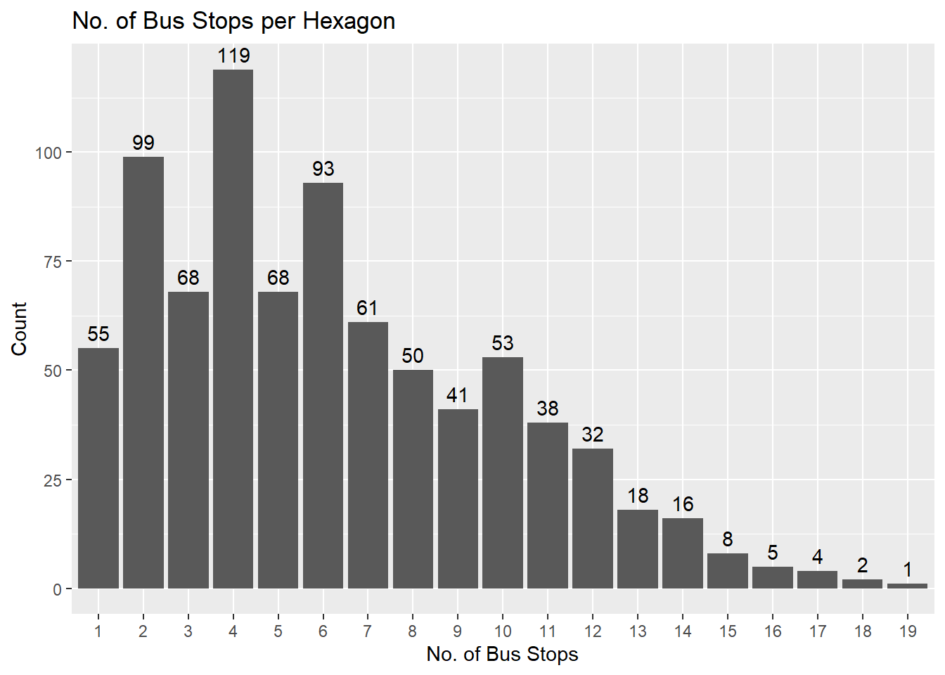
In the bar chart below, it is evident that the distribution of bus stops per hexagon is right-skewed. While one hexagon contains as many as 19 bus stops, the majority have fewer than 10 bus stops.

Show the code

ggplot(area_hexagon_grid, 
       aes(x= as.factor(busstops)))+   
  geom_bar()+   
  ggtitle("No. of Bus Stops per Hexagon") +
  geom_text(aes(label = after_stat(count)), 
            stat = "count", 
            vjust = -0.5, 
            colour = "black")+
  labs(x= "No. of Bus Stops", y = "Count")

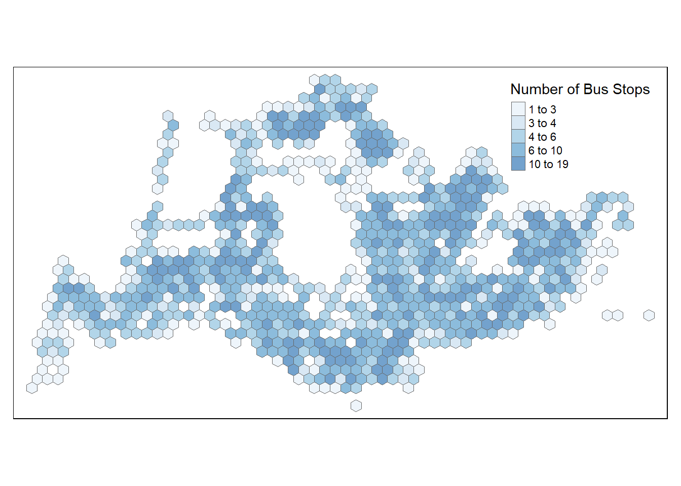
Lastly, using tm_shape from tmap package, we can quickly visualise the results of the hexagon grids we have created.

Show the code

tmap_mode ("plot")
tm_shape(area_hexagon_grid)+
  tm_fill(
    col = "busstops",
    palette = "Blues",
    style = "quantile",
    title = "Number of Bus Stops",
    id = "grid_id",
    showNA = FALSE,
    alpha = 0.6,
    popup.format = list(
      grid_id = list(format = "f", digits = 0)
    )
  )+
  tm_borders(col = "grey40", lwd = 0.7)

3.3 Geospatial Data Wrangling

3.3.1 Combining Busstop and Hexagons

Code chunk below populates the grid ID (i.e. grid_id) of area_hexagon_grid sf data frame into busstop sf data frame using the following functions:

• st_intersection() is used to perform point and polygon overly and the output will be in point sf object.

• select() of dplyr package is then use to retain preferred variables from the data frames.

• st_stop_geometry() removes the geometry data to manipulate it like a regular dataframe using tidyr and dplyr functions

bs_wgrids <- st_intersection(busstop, area_hexagon_grid) %>% 
  dplyr::select(BUS_STOP_N,BUS_ROOF_N,LOC_DESC, grid_id) %>% 
  st_drop_geometry

Before we proceed, let’s perform a duplicates check on bs_wgrids.

duplicate <- bs_wgrids %>%
  group_by_all() %>%
  filter(n()>1) %>%
  ungroup()

duplicate

# A tibble: 0 × 4
# ℹ 4 variables: BUS_STOP_N <chr>, BUS_ROOF_N <chr>, LOC_DESC <chr>,
#   grid_id <int>

Results showed that there are no duplicated records.

3.3.2 Populate Passenger Volume data with Grid IDs

Next, we are going to append the Grid IDs based on origin bus stops from bs_wgrids data frame onto WDMpeak data frame. But before that, ensure that BUS_STOP_N of bs_wgrids is also in factor data type.

bs_wgrids$BUS_STOP_N  <- as.factor(bs_wgrids$BUS_STOP_N)


od_data <- left_join(WDMpeak , bs_wgrids,
            by = c("ORIGIN_PT_CODE" = "BUS_STOP_N")) %>% 
  rename(ORIGIN_BS = ORIGIN_PT_CODE,
         ORIGIN_GRID = grid_id,
         ORIGIN_DESC = LOC_DESC,
         DESTIN_BS = DESTINATION_PT_CODE)

Next, we will update od_data data frame with the Grid IDs of destination bus stops.

od_data <- left_join(od_data , bs_wgrids,
            by = c("DESTIN_BS" = "BUS_STOP_N")) %>% 
           rename(DESTIN_GRID = grid_id,
                  DESTIN_DESC = LOC_DESC)

glimpse(od_data)

Rows: 242,208
Columns: 9
Groups: ORIGIN_BS [5,029]
$ ORIGIN_BS    <fct> 01012, 01012, 01012, 01012, 01012, 01012, 01012, 01012, 0…
$ DESTIN_BS    <fct> 01112, 01113, 01121, 01211, 01311, 07371, 60011, 60021, 6…
$ TRIPS        <dbl> 290, 118, 77, 118, 165, 14, 30, 16, 35, 26, 2, 8, 1, 2, 2…
$ BUS_ROOF_N.x <chr> "B03", "B03", "B03", "B03", "B03", "B03", "B03", "B03", "…
$ ORIGIN_DESC  <chr> "HOTEL GRAND PACIFIC", "HOTEL GRAND PACIFIC", "HOTEL GRAN…
$ ORIGIN_GRID  <int> 1334, 1334, 1334, 1334, 1334, 1334, 1334, 1334, 1334, 133…
$ BUS_ROOF_N.y <chr> "B07", "B09", "B11", "B13", "B01", "B01", "B01", "B03", "…
$ DESTIN_DESC  <chr> "OPP BUGIS STN EXIT C", "BUGIS STN EXIT B", "STAMFORD PR …
$ DESTIN_GRID  <int> 1354, 1354, 1392, 1392, 1411, 1411, 1393, 1431, 1450, 143…

The code chunk below allows us to check for duplicates to prevent double counting. The results indicate that there are no duplicates found.

duplicate2 <- od_data %>%
  group_by_all() %>%
  filter(n()>1) %>%
  ungroup()

duplicate2

# A tibble: 0 × 9
# ℹ 9 variables: ORIGIN_BS <fct>, DESTIN_BS <fct>, TRIPS <dbl>,
#   BUS_ROOF_N.x <chr>, ORIGIN_DESC <chr>, ORIGIN_GRID <int>,
#   BUS_ROOF_N.y <chr>, DESTIN_DESC <chr>, DESTIN_GRID <int>

Next, the code chunk below removes rows with missing data using drop_na() and aggregates the total passenger trips at each origin-destination grid level with group_by() and summarise(). ORIGIN_nBS and DESTIN_nBS counts the number of bus stops, while ORIGIN_DESC and DESTIN_DESC provides the descriptions of each of the bus stops at origin and destination grids respectively.

od_data <- od_data %>%
  drop_na() %>%
  group_by(ORIGIN_GRID, DESTIN_GRID) %>%
  summarise(MORNING_PEAK = sum(TRIPS),
            ORIGIN_nBS = n_distinct(ORIGIN_BS),
            ORIGIN_DESC = str_c(unique(ORIGIN_DESC), collapse = ", "),
            DESTIN_nBS = n_distinct(DESTIN_BS),
            DESTIN_DESC = str_c(unique(DESTIN_DESC), collapse = ", ")) %>%
  ungroup()

Our resulting OD Matrix organises the commuter flows for weekday morning peak period in a column-wise format, with origin_grid representing the from and destin_grid representing the to. There are a total of 65,559 unique origin grid to destination grid combinations.

Show the code

DT::datatable(od_data,
              options = list(pageLength = 5),
              rownames = FALSE)

4 Visualising Spatial Interaction

Origin-destination flow maps are a popular option to visualise connections between different spatial locations. It reflects the relationships/flows between locations and are created by monitoring movements. In our analysis, we can use OD flows to identify the patterns of bus ridership during weekday mornings.

4.1 Identifying Inter- & Intra-Zonal Flows

Intrazonal travels are considered localised and short duration trips within a transportation analysis zone (i.e. within a hexagon). For our analysis, we will be separating them.

To do that, we create a new column in the od_data dataframe called Zone_Type using mutate() that labels each row as either “Intrazone” or “Interzone” based on whether the ORIGIN_GRID and DESTIN_GRID are the same or different.

od_data <- od_data %>%
  mutate(Zone_Type = ifelse(ORIGIN_GRID == DESTIN_GRID, "intrazone", "interzone"))

There are 623 combinations of intra-zonal travels and 64,936 combinations of inter-zonal travels during the weekday morning peak period based on our dataset.

table(od_data$Zone_Type)

interzone intrazone 
    64936       623 

4.2 Interzonal OD Flow Distribution

In the code chunk below, we use filter() to identify the inter-data before using summary() to evaulate the distribution of data.

Show the code

od_interzone <- od_data %>%
  filter(Zone_Type == "interzone")

quantile(od_interzone$MORNING_PEAK, 
         probs = seq(0, 1.0, by = .05))

   0%    5%   10%   15%   20%   25%   30%   35%   40%   45%   50%   55%   60% 
    1     1     2     3     5     7    11    15    21    28    37    50    67 
  65%   70%   75%   80%   85%   90%   95%  100% 
   90   124   174   252   388   658  1399 77433 

From the summary statistics provided above, we observe that the minimum number of passenger trips for each interzonal combination of origin and destination bus stop is 1. The maximum number of trips recorded is 77,433 passengers, noted during the weekday morning peak period. Additionally, the 90th percentile for passenger trips stands at 174, indicating a highly right-skewed distribution.

4.2 Creating Interzonal Flow Lines

Desire lines visually represent the connections between originating and destination hexagons using straight lines. The od2line() function of stplanr package is utilized to create these lines. The width of each desire line is proportional to number of passenger trips, i.e. thicker lines would represent higher ridership.

# Creating centroids representing desire line start and end points
flowLine <- od2line(flow = od_interzone, 
                    zones = area_hexagon_grid,
                    zone_code = "grid_id")

Since there are 65,559 different flow lines resulting from combinations of origin to destination hexagons, an excess of intersecting lines can cause visual clutter and obscure analysis. Considering that the 90th percentile is 658, we will focus on inter-zonal flows with the top 10% of ridership.

Show the code

tmap_mode("view")
tmap_options(check.and.fix = TRUE)

#tm_basemap("OneMapSG.Grey") +
tm_basemap("OpenStreetMap") +
tm_shape(mpsz) +
  tm_polygons(col='#C2D3CC', border.alpha = 0.1, alpha = 0.3) +
tm_shape(area_hexagon_grid) +
  tm_fill(alpha=0.7, 
          palette="RdBu") + 
  tm_borders(alpha = 0.5)+
flowLine %>%  
  filter(MORNING_PEAK >= 659) %>% 
tm_shape() +
  tm_lines(lwd = "MORNING_PEAK",
           style = "quantile",
           scale = c(0.1, 1, 3, 5, 7, 10),
           n = 6,
           alpha = 0.3,
           lines.lwd = "all",
           popup.vars = c("No. of Bus Stops at Origin: " = "ORIGIN_nBS",
                         "Descriptions of Bus Stops at Origin: " = "ORIGIN_DESC",
                         "No. of Bus Stops at Destination: " = "DESTIN_nBS",
                         "Descriptions of Bus Stops at Destination: " = "DESTIN_DESC",
                         "No. of Passenger Trips :" = "MORNING_PEAK"))

Show the code

#tm_view(set.zoom.limits = c(11,14))

The map reveals that Yew Tee, Woodlands, and Yishun dominate inter-zonal bus ridership during weekday mornings, with notably wider desire lines. Key routes include travel within Yew Tee, between Woodlands Checkpoint and Woodlands MRT Station, as well as within Woodlands and Yishun. Interestingly, though broad, these desire lines are relatively short, often indicating bus travel to neighboring hexagons. This suggests a higher demand for feeder bus services in these areas during weekday mornings. Areas such as Boon Lay, Bedok, Choa Chu Kang, Clementi, Tampines, Pasir Ris, and Serangoon also display high concentrations and variations of desire lines with neighboring hexagons, indicating higher ridership within these areas.

Furthermore, longer desire lines between the North and East (i.e., Woodlands and Changi) suggest passengers’ willingness to travel longer distances to their destinations.

While OD flows provide valuable insights by quickly visualizing travel patterns, it is beneficial to complement them with other forms of analysis, such as spatial interaction models, for a more comprehensive understanding of the factors affecting urban commuting flow.

5 Computing Distance Matrix

A distance matrix is a two-dimensional array containing the distances between different locations. In our analysis, we can use a distance matrix to calculate the distance passengers are willing to travel by bus to get to their destinations.

5.1 Converting from sf data.table to SpatialPolygonsDataFrame

Firstly, as.Spatial() will be used to convert area_hexagon_grid from sf tibble data frame to SpatialPolygonsDataFrame of sp object as shown in the code chunk below.

hexgrid_sp <- as(area_hexagon_grid, "Spatial")
hexgrid_sp

class       : SpatialPolygonsDataFrame 
features    : 831 
extent      : 3595.122, 48595.12, 26049.09, 50297.8  (xmin, xmax, ymin, ymax)
crs         : +proj=tmerc +lat_0=1.36666666666667 +lon_0=103.833333333333 +k=1 +x_0=28001.642 +y_0=38744.572 +ellps=WGS84 +towgs84=0,0,0,0,0,0,0 +units=m +no_defs 
variables   : 2
names       : grid_id, busstops 
min values  :      21,        1 
max values  :    2267,       19 

5.2 Computing Distance Matrix

Next, spDists() of sp package will be used to compute the Euclidean distance between the centroids of the planning subzones. spDists returns a full matrix of distances in the metric of the points if longlat=FALSE, or in kilometers if longlat=TRUE. With 831 hexagons, the return results will produce a 831 by 831 matrix of distance between each hexagon.

dist <- spDists(hexgrid_sp, 
                longlat = FALSE)

head(dist, n=c(6, 6))

         [,1]     [,2]     [,3]     [,4]     [,5]     [,6]
[1,]    0.000  750.000 3269.174 1500.000 2704.163 3968.627
[2,]  750.000    0.000 2598.076  750.000 1984.313 3269.174
[3,] 3269.174 2598.076    0.000 1984.313  750.000  750.000
[4,] 1500.000  750.000 1984.313    0.000 1299.038 2598.076
[5,] 2704.163 1984.313  750.000 1299.038    0.000 1299.038
[6,] 3968.627 3269.174  750.000 2598.076 1299.038    0.000

The resulting output is a matrix object class.

Note that column headers and row headers are not labeled with the grid IDs, in the next step, we rename the headers for better clarity.

grid_id <- area_hexagon_grid$grid_id

colnames(dist) <- paste0(grid_id)
rownames(dist) <- paste0(grid_id)

head(dist, n=c(6, 6))

         21       40       42       60       61       62
21    0.000  750.000 3269.174 1500.000 2704.163 3968.627
40  750.000    0.000 2598.076  750.000 1984.313 3269.174
42 3269.174 2598.076    0.000 1984.313  750.000  750.000
60 1500.000  750.000 1984.313    0.000 1299.038 2598.076
61 2704.163 1984.313  750.000 1299.038    0.000 1299.038
62 3968.627 3269.174  750.000 2598.076 1299.038    0.000

Notice that the column and row names have been updated to the grid IDs.

5.3 Pivoting Distance Value by Grid ID

Next, we will pivot the distance matrix into a long table by using the row and column grid IDs using melt() of the reshape2 package, as shown in the code chunk below.

distPair <- melt(dist) %>%
  rename(dist = value,
         orig = Var1,
         dest = Var2)

head(distPair, 5)

  orig dest     dist
1   21   21    0.000
2   40   21  750.000
3   42   21 3269.174
4   60   21 1500.000
5   61   21 2704.163

Notice that the within-zone distance is 0.

5.4 Updating Intra-Zonal Distances

In this section, we are going to append a constant value to replace the intra-zonal distance of 0.

First, we will select and find out the minimum value of the distance by using summary().

distPair %>%
  filter(dist > 0) %>%
  summary()

      orig           dest           dist      
 Min.   :  21   Min.   :  21   Min.   :  750  
 1st Qu.: 789   1st Qu.: 789   1st Qu.: 8250  
 Median :1200   Median :1200   Median :13269  
 Mean   :1150   Mean   :1150   Mean   :14135  
 3rd Qu.:1529   3rd Qu.:1529   3rd Qu.:18929  
 Max.   :2267   Max.   :2267   Max.   :44680  

Next, an arbitrary constant distance value of 100m is added into intra-zones distance

distPair$dist <- ifelse(distPair$dist == 0,
                        100, 
                        distPair$dist)

The code chunk below will be used to check the result using summary().

summary(distPair)

      orig           dest           dist      
 Min.   :  21   Min.   :  21   Min.   :  100  
 1st Qu.: 789   1st Qu.: 789   1st Qu.: 8250  
 Median :1200   Median :1200   Median :13269  
 Mean   :1150   Mean   :1150   Mean   :14119  
 3rd Qu.:1529   3rd Qu.:1529   3rd Qu.:18929  
 Max.   :2267   Max.   :2267   Max.   :44680  

5.5 Combining passenger volume data with distance value

Let’s convert the origin and destination grid data in od_data and distPair into factor data type before we combine passenger volume data from od_data and distance from distPair using left_join().

od_data$ORIGIN_GRID  <- as.factor(od_data$ORIGIN_GRID)
od_data$DESTIN_GRID  <- as.factor(od_data$DESTIN_GRID)

distPair$orig  <- as.factor(distPair$orig)
distPair$dest  <- as.factor(distPair$dest)

flow_data <- od_data %>%
  left_join (distPair,
             by = c("ORIGIN_GRID" = "orig",
                    "DESTIN_GRID" = "dest"))

glimpse(flow_data)

Rows: 65,559
Columns: 9
$ ORIGIN_GRID  <fct> 21, 21, 21, 21, 21, 21, 40, 40, 40, 40, 40, 40, 40, 40, 4…
$ DESTIN_GRID  <fct> 61, 79, 116, 140, 159, 160, 21, 61, 78, 80, 116, 136, 140…
$ MORNING_PEAK <dbl> 1, 1, 4, 3, 93, 1, 1, 2, 1, 2, 3, 1, 2, 40, 1, 1, 3, 2, 2…
$ ORIGIN_nBS   <int> 1, 1, 1, 1, 1, 1, 1, 1, 1, 1, 1, 1, 1, 1, 1, 1, 1, 1, 1, …
$ ORIGIN_DESC  <chr> "AFT TUAS STH BLVD", "AFT TUAS STH BLVD", "AFT TUAS STH B…
$ DESTIN_nBS   <int> 1, 1, 1, 1, 1, 1, 1, 1, 1, 1, 1, 1, 1, 1, 1, 1, 3, 1, 1, …
$ DESTIN_DESC  <chr> "THE INDEX", "ABBOTT", "AFT TUAS STH ST 7", "BEF TUAS AVE…
$ Zone_Type    <chr> "interzone", "interzone", "interzone", "interzone", "inte…
$ dist         <dbl> 2704.163, 2250.000, 1984.313, 6873.864, 7611.669, 8842.37…

5.6 Distance Distribution

Show the code

quantile(flow_data$dist, 
         probs = seq(0, 1.0, by = .1))

       0%       10%       20%       30%       40%       50%       60%       70% 
  100.000  1500.000  2598.076  3436.932  4500.000  5408.327  6538.348  7937.254 
      80%       90%      100% 
 9807.523 12346.558 24784.067 

From the summary statistics above, the minimum number of passenger trips for each combination of origin and destination bus stop is 100m, which is the arbitrary intrazonal travel distance we have set. The maximum observed is 24,784m.

Show the code

# Extract column
distWDM_distance <- flow_data$dist
# Calculate mean 
distWDM_distance_mean <- mean(distWDM_distance)

ggplot(
    data = data.frame(distWDM_distance),
    aes(x = distWDM_distance)
  ) +
  geom_histogram(
    bins = 20, 
    color = "#FFFCF9", 
    fill = "black",
    alpha = .3
  ) +
  # Add line for mean
  geom_vline(
    xintercept = distWDM_distance_mean, 
    color = "#595DE5", 
    linetype = "dashed", 
    linewidth = 1
  ) +
  scale_x_continuous(breaks = pretty(distWDM_distance, n = 10))+
  # Add line annotations
  annotate(
    "text", 
    x = 9000, 
    y = 7500,
    label = paste("Mean =", round(distWDM_distance_mean, 3)),
    color = "#595DE5",
    size = 3
  ) +
  labs(
    title = "Weekday Morning Peak",
    x = "Distance of Bus Trips",
    y = "Frequency"
  ) 

5.6 Visualise Flow Lines

Since the 90th percentile of the distance traveled is 12,346.558m, we will filter the data for distances greater than 12,347m to analyse the top 10% of the longest distances traveled.

Show the code

# Creating centroids representing desire line start and end points
flowLine2 <- od2line(flow = flow_data, 
                    zones = area_hexagon_grid,
                    zone_code = "grid_id")

tmap_mode("view")
tmap_options(check.and.fix = TRUE)

#tm_basemap("OneMapSG.Grey") +
tm_basemap("OpenStreetMap") +
tm_shape(mpsz) +
  tm_polygons(alpha = 0) +
  tm_borders(alpha = 0.5)+
tm_shape(area_hexagon_grid) +
  tm_fill(alpha=0.7, 
          palette="RdBu") + 
  tm_borders(alpha = 0.5)+
flowLine2 %>%  
  filter(dist >= 12347) %>% 
tm_shape() +
  tm_lines(lwd = "MORNING_PEAK",
           style = "quantile",
           scale = c(0.1, 1, 3, 5, 7, 10),
           n = 6,
           alpha = 0.3,
           lines.lwd = "all",
           popup.vars = c("No. of Bus Stops at Origin: " = "ORIGIN_nBS",
                         "Descriptions of Bus Stops at Origin: " = "ORIGIN_DESC",
                         "No. of Bus Stops at Destination: " = "DESTIN_nBS",
                         "Descriptions of Bus Stops at Destination: " = "DESTIN_DESC",
                         "No. of Passenger Trips :" = "MORNING_PEAK"))

Show the code

#tm_view(set.zoom.limits = c(11,14))

The plot below reveals that longer travel distances predominantly occur between North and North-East regions (i.e., Woodlands/Yishun and Punggol), North and East (Woodlands and Tampines), West and South (Choa Chu Kang/Bukit Panjang and the Town area), and North and South (Yishun and the Town area). These patterns may reflect commuting trends between residential and commercial areas, suggesting that significant portion of the population undertake considerable daily commutes.

The sparseness of flow lines seen in the West-end also ascertains the trends noted in our previous Take-Home Exercise 1, where low-low autocorrelation were noted in that area.

In the subsequent sections, we explore the potential factors that could attract or propel passengers to travel by bus from one location to another. This exploration will include examining various urban elements such as the proximity to key amenities like schools, shopping centers, and employment hubs. Understanding these elements can provide valuable insights into improving public transportation systems and urban planning strategies.

6 Preparing Origin and Destination Attributes

The following information is used to derive propulsive/attractiveness variables:

1. Business, FinServ, Leisure&Recreation and Retails are geospatial data sets of the locations of business establishments, entertainments, food and beverage outlets, financial centres, leisure and recreation centres, retail and services stores/outlets.

2. Schools: This data set contains directory and general information of schools in Singapore, obtained from data.gov.

3. HDB: This data set is the geocoded version of HDB Property Information data from data.gov. The data set is prepared using September 2021 data.

Train Station Exits

trainstationexits contains the MRT station names and exits along with their respective point geometries in CRS SVY21.

Train stations exits reflect the intermodal connections with bus stops. In the context of attractiveness, these stations can be seen as destinations that attract passengers, including those who might transit to/from these stations by bus. The data can also indicate the propulsiveness aspect – how these stations act as origins for passengers who leave the MRT stations and then proceed to their final destinations via other modes of transportation like buses.

Step 1: Import shapefile

st_read() function of the sf package enables us to import the file into RStudio.

trainstationexits <- st_read(dsn = "data/geospatial",
                   layer = "Train_Station_Exit_layer") %>% 
  st_transform(crs = 3414)

Reading layer `Train_Station_Exit_layer' from data source 
  `C:\kytjy\ISSS624\Take-Home_Ex\Take-Home_Ex2\data\geospatial' 
  using driver `ESRI Shapefile'
Simple feature collection with 565 features and 2 fields
Geometry type: POINT
Dimension:     XY
Bounding box:  xmin: 6134.086 ymin: 27499.7 xmax: 45356.36 ymax: 47865.92
Projected CRS: SVY21

Notice there are 565 train station exits in total.

A quick check for duplicates revealed that there are cases where same station names and exit codes have different geometries. In the absence of further information, it is prudent to retain all these details, as they might represent cases where lifts and escalators at the exits are located at different points.

trainstationexits %>%
  group_by(stn_name, exit_code) %>%
  filter(n() > 1) %>%
  ungroup() %>%
  arrange(stn_name, exit_code) %>% 
  kable()

stn_name	exit_code	geometry
BEDOK NORTH MRT STATION	Exit B	POINT (37542.44 35150.99)
BEDOK NORTH MRT STATION	Exit B	POINT (37550.39 35173.81)
BUKIT PANJANG MRT STATION	Exit A	POINT (20054.56 40109.33)
BUKIT PANJANG MRT STATION	Exit A	POINT (19795.81 40301.42)
BUKIT PANJANG MRT STATION	Exit A	POINT (20066.96 40082.6)
CHOA CHU KANG MRT STATION	Exit A	POINT (18121.99 40819.65)
CHOA CHU KANG MRT STATION	Exit A	POINT (18122.31 40816.19)
CHOA CHU KANG MRT STATION	Exit C	POINT (18117.61 40853.37)
CHOA CHU KANG MRT STATION	Exit C	POINT (18112.29 40852.68)
CHOA CHU KANG MRT STATION	Exit D	POINT (18084.87 40849.96)
CHOA CHU KANG MRT STATION	Exit D	POINT (18072.23 40812.88)
EXPO MRT STATION	Exit A	POINT (42314.55 35278.98)
EXPO MRT STATION	Exit A	POINT (42302.73 35296.8)
HARBOURFRONT MRT STATION	Exit A	POINT (26569.87 27614.83)
HARBOURFRONT MRT STATION	Exit A	POINT (26797.06 27512.2)
UPPER CHANGI MRT STATION	Exit A	POINT (42246.13 36002.08)
UPPER CHANGI MRT STATION	Exit A	POINT (42205.19 36018.15)

Step 2: Point-in-Polygon Count Process

Next, we will count the number of train station exits located inside each hexagon and include this as a variable in area_hexagon_grid table.

area_hexagon_grid$`COUNT_TRAINSTATIONEXIT`<- lengths(
  st_intersects(
    area_hexagon_grid, trainstationexits))

sum(area_hexagon_grid$COUNT_TRAINSTATIONEXIT)

[1] 560

The 5 train station exits not accounted for could be in areas outside hexagons where there are no bus stop.

Summary statistics indicate that a maximum of 13 train station exits are located within a single hexagon, while at least 75% of the hexagons do not contain any exits.

summary(area_hexagon_grid$COUNT_TRAINSTATIONEXIT)

   Min. 1st Qu.  Median    Mean 3rd Qu.    Max. 
 0.0000  0.0000  0.0000  0.6739  0.0000 13.0000 

Let’s visualise where the bus stops are located, alongside the top 5% of ridership, to see if we can identify any discernible patterns.

Show the code

tmap_mode("plot")
tm_shape(mpsz) +
  tm_polygons(col='#C2D3CC', border.alpha = 0.1, alpha = 0.3) +
tm_shape(area_hexagon_grid) +
  tm_fill(
    col="COUNT_TRAINSTATIONEXIT",
    style="pretty",
    palette="Blues",
    alpha=0.7) +
  tm_borders(alpha = 0.5) +
flowLine %>%  
  filter(MORNING_PEAK >= 1399) %>% 
tm_shape() +
  tm_lines(lwd = "MORNING_PEAK",
           style = "quantile",
           scale = c(0.1, 1, 3, 5, 7, 10),
           n = 6,
           alpha = 0.1)+
    tm_layout(legend.text.size = 0.6,
              legend.title.size=0.6)

Business

business contains the details of various businesses from SMEs to bigger groups like Pan Pacific, as well as the respective point geometries in CRS SVY21.

Businesses serve as significant attractors in a city. They draw people to these locations, primarily for work purposes. The presence and density of businesses in an area can significantly influence the flow of commuters, making it a measure of attractiveness.

Step 1: Import shapefile

Show the code

business <- st_read(dsn = "data/geospatial",
                      layer = "Business") %>%
          st_transform(crs = 3414)

Reading layer `Business' from data source 
  `C:\kytjy\ISSS624\Take-Home_Ex\Take-Home_Ex2\data\geospatial' 
  using driver `ESRI Shapefile'
Simple feature collection with 6550 features and 3 fields
Geometry type: POINT
Dimension:     XY
Bounding box:  xmin: 3669.148 ymin: 25408.41 xmax: 47034.83 ymax: 50148.54
Projected CRS: SVY21 / Singapore TM

Note that there are 6550 business in our dataset in total.

Our duplicate check showed KEPPEL DISTRIPARK is included twice in the dataset. We remove this to prevent double-counting.

business %>%
  group_by_all() %>%
  filter(n() > 1) %>%
  ungroup() %>%
  arrange(POI_NAME) %>% 
  kable()

POI_NAME	POI_ST_NUM	POI_ST_NAM	geometry
KEPPEL DISTRIPARK	511	KG BAHRU RD	POINT (27455.94 28233.69)
KEPPEL DISTRIPARK	511	KG BAHRU RD	POINT (27455.94 28233.69)

business <- unique(business)

Note that the number of records for business is has decreased from 6550 to 6549.

Step 2: Point-in-Polygon Count Process

Next, we will count the number of business in each hexagon and include this as a variable in area_hexagon_grid table.

area_hexagon_grid$`COUNT_BIZ`<- lengths(
  st_intersects(
    area_hexagon_grid, business))

Summary statistics below show that less than half of the hexagons do not contain any businesses, while in contrast, a single hexagon houses as many as 97 businesses.

summary(area_hexagon_grid$COUNT_BIZ)

   Min. 1st Qu.  Median    Mean 3rd Qu.    Max. 
  0.000   0.000   1.000   7.298   7.000  97.000 

Let’s visualise where the businesses are located, alongside the top 5% of ridership, to see if we can identify any discernible patterns.

Show the code

tmap_mode("plot")
tm_shape(mpsz) +
  tm_polygons(col='#C2D3CC', border.alpha = 0.1, alpha = 0.3) +
tm_shape(area_hexagon_grid) +
  tm_fill(
    col="COUNT_BIZ",
    style="pretty",
    palette="Blues",
    alpha=0.7) +
  tm_borders(alpha = 0.5) +
flowLine %>%  
  filter(MORNING_PEAK >= 1399) %>% 
tm_shape() +
  tm_lines(lwd = "MORNING_PEAK",
           style = "quantile",
           scale = c(0.1, 1, 3, 5, 7, 10),
           n = 6,
           alpha = 0.1)+
    tm_layout(legend.text.size = 0.6,
              legend.title.size=0.6)

No consistent patterns are evident when comparing the number of businesses in a grid with the top 5% of ridership. In the far West, despite a significant presence of businesses, the passenger volume does not rise correspondingly. In contrast, areas like Changi, Woodlands, the Central Business District, and Geylang, which have higher numbers of business units, also experience greater passenger volumes.

Financial Centres

finserv contains the details of various financial centres, as well as the respective point geometries in CRS SVY21.

Financial service locations often represent significant employment centers, especially in urban and commercial areas. Many people travel to these locations for work, making them important attractors during morning peak hours. In addition, financial services typically adhere to standard office hours, which aligns well with the morning peak period of bus ridership, as a large proportion of employees would be traveling to work during this time.

Step 1: Import shapefile

Show the code

finserv <- st_read(dsn = "data/geospatial",
                      layer = "FinServ") %>%
          st_transform(crs = 3414)

Reading layer `FinServ' from data source 
  `C:\kytjy\ISSS624\Take-Home_Ex\Take-Home_Ex2\data\geospatial' 
  using driver `ESRI Shapefile'
Simple feature collection with 3320 features and 3 fields
Geometry type: POINT
Dimension:     XY
Bounding box:  xmin: 4881.527 ymin: 25171.88 xmax: 46526.16 ymax: 49338.02
Projected CRS: SVY21 / Singapore TM

Note that there are 3320 locations of financial services in our dataset in total.

Similarly, we remove duplicates by retaining the unique observations to prevent double-counting. This reduces the number of financial services locations from 3320 to 3058.

finserv <- unique(finserv)

Step 2: Point-in-Polygon Count Process

Next, we will count the number of financial services in each hexagon and include this as a variable in area_hexagon_grid table.

area_hexagon_grid$`COUNT_FS`<- lengths(
  st_intersects(
    area_hexagon_grid, finserv))

The summary statistics reveal that up to 130 financial services locations can be found within a single hexagon, with less than half of the hexagons are devoid of any such locations.

summary(area_hexagon_grid$COUNT_FS)

   Min. 1st Qu.  Median    Mean 3rd Qu.    Max. 
  0.000   0.000   1.000   3.626   4.000 130.000 

Let’s visualise where these are located, alongside the top 5% of ridership, to see if we can identify any discernible patterns.

Show the code

tmap_mode("plot")
tm_shape(mpsz) +
  tm_polygons(col='#C2D3CC', border.alpha = 0.1, alpha = 0.3) +
tm_shape(area_hexagon_grid) +
  tm_fill(
    col="COUNT_FS",
    style="pretty",
    palette="Blues",
    alpha=0.7) +
  tm_borders(alpha = 0.5) +
flowLine %>%  
  filter(MORNING_PEAK >= 1399) %>% 
tm_shape() +
  tm_lines(lwd = "MORNING_PEAK",
           style = "quantile",
           scale = c(0.1, 1, 3, 5, 7, 10),
           n = 6,
           alpha = 0.1)+
    tm_layout(legend.text.size = 0.6,
              legend.title.size=0.6)

Similarly, the relationship between ridership and the count of financial services is not particularly obvious. High ridership is observed outside the Central Business District area, where financial services are concentrated.

Leisure & Recreation Centres

recs includes information on various leisure and recreation centers, such as playgrounds, parks, and fitness centers. It also contains their respective point geometries in the CRS SVY21.

Recreational facilities could be popular for early morning workouts and might be an attractor for the morning crowd.

Step 1: Import shapefile

Show the code

recs <- st_read(dsn = "data/geospatial",
                      layer = "Liesure&Recreation") %>%
          st_transform(crs = 3414)

Reading layer `Liesure&Recreation' from data source 
  `C:\kytjy\ISSS624\Take-Home_Ex\Take-Home_Ex2\data\geospatial' 
  using driver `ESRI Shapefile'
Simple feature collection with 1217 features and 30 fields
Geometry type: POINT
Dimension:     XY
Bounding box:  xmin: 6010.495 ymin: 25134.28 xmax: 48439.77 ymax: 50078.88
Projected CRS: SVY21 / Singapore TM

Note that there are 1217 locations of leisure and recreational centres in our dataset in total.

The results from the duplicate check show that no duplicates were found

finserv %>%
  group_by_all() %>%
  filter(n() > 1) %>%
  ungroup() %>%
  arrange(POI_NAME) %>% 
  kable()

POI_NAME	POI_ST_NUM	POI_ST_NAM	geometry

Step 2: Point-in-Polygon Count Process

Next, we will count the number of facilities in each hexagon and include this as a variable in area_hexagon_grid table.

area_hexagon_grid$`COUNT_RECS`<- lengths(
  st_intersects(
    area_hexagon_grid, recs))

The summary statistics indicate that, on average, a single leisure and recreational facility is found within each hexagon, although the highest number recorded in a hexagon is 41.

summary(area_hexagon_grid$COUNT_RECS)

   Min. 1st Qu.  Median    Mean 3rd Qu.    Max. 
  0.000   0.000   0.000   1.312   1.000  41.000 

Let’s visualise where these are located, alongside the top 5% of ridership, to see if we can identify any discernible patterns.

Show the code

tmap_mode("plot")
tm_shape(mpsz) +
  tm_polygons(col='#C2D3CC', border.alpha = 0.1, alpha = 0.3) +
tm_shape(area_hexagon_grid) +
  tm_fill(
    col="COUNT_RECS",
    style="pretty",
    palette="Blues",
    alpha=0.7) +
  tm_borders(alpha = 0.5) +
flowLine %>%  
  filter(MORNING_PEAK >= 1399) %>% 
tm_shape() +
  tm_lines(lwd = "MORNING_PEAK",
           style = "quantile",
           scale = c(0.1, 1, 3, 5, 7, 10),
           n = 6,
           alpha = 0.1)+
    tm_layout(legend.text.size = 0.6,
              legend.title.size=0.6)

Similarly, the relationship between the number of bus trips and the presence of leisure and recreational centers is not consistently clear across all areas. Locations such as the CBD, Yishun, and Tampines, which have a higher concentration of recreational centers, do indeed experience higher ridership.

Retail

retail includes information on various retail and services stores/outlets, along with their respective point geometries in the CRS SVY21.

Retail locations can be significant attractors in the morning, particularly as employment destinations for people who work in these retail and service outlets. Some retail services, like coffee shops, breakfast spots, and convenience stores, might attract early morning customers, including commuters heading to work.

Step 1: Import shapefile

Show the code

retail <- st_read(dsn = "data/geospatial",
                  layer = "Retails") %>%
          st_transform(crs = 3414)

Reading layer `Retails' from data source 
  `C:\kytjy\ISSS624\Take-Home_Ex\Take-Home_Ex2\data\geospatial' 
  using driver `ESRI Shapefile'
Simple feature collection with 37635 features and 3 fields
Geometry type: POINT
Dimension:     XY
Bounding box:  xmin: 4737.982 ymin: 25171.88 xmax: 48265.04 ymax: 50135.28
Projected CRS: SVY21 / Singapore TM

Note that there are 37635 retail locations in our dataset in total.

Similarly, we remove duplicates to prevent double-counting. This reduces the number of retail services locations from 37,635 to 37,460.

retail <- unique(retail)

Step 2: Point-in-Polygon Count Process

Next, we will count the number of retail centres in each hexagon and include this as a variable in area_hexagon_grid table.

area_hexagon_grid$`COUNT_RETAIL`<- lengths(
  st_intersects(
    area_hexagon_grid, retail))

The summary statistics reveal that, on average, 44 retail and service centers can be located within a single hexagon, with the maximum number reaching 1669.

summary(area_hexagon_grid$COUNT_RETAIL)

   Min. 1st Qu.  Median    Mean 3rd Qu.    Max. 
   0.00    1.00    8.00   43.99   36.50 1669.00 

Let’s visualise where these are located, alongside the top 5% of ridership, to see if we can identify any discernible patterns.

Show the code

tmap_mode("plot")
tm_shape(mpsz) +
  tm_polygons(col='#C2D3CC', border.alpha = 0.1, alpha = 0.3) +
tm_shape(area_hexagon_grid) +
  tm_fill(
    col="COUNT_RETAIL",
    style="pretty",
    palette="Blues",
    alpha=0.7) +
  tm_borders(alpha = 0.5) +
flowLine %>%  
  filter(MORNING_PEAK >= 1399) %>% 
tm_shape() +
  tm_lines(lwd = "MORNING_PEAK",
           style = "quantile",
           scale = c(0.1, 1, 3, 5, 7, 10),
           n = 6,
           alpha = 0.1)+
    tm_layout(legend.text.size = 0.6,
              legend.title.size=0.6)

Significant passenger flows are observed in the Town area where the retail count is high. However, high passenger flows are also noted in areas where retail units are not as abundant, such as Woodlands and Jurong.

Schools

The schools data is taken from School Directory and Information as of March 2022 from data.gov.

Schools significantly impact local transit patterns, especially during morning and afternoon peak hours. Regular travel routines of students, teachers, and staff create predictable demand, with a high volume of commuters contributing substantially to local transit ridership, making it a critical attractor. This effect is particularly pronounced on bus routes serving school areas, where the demand for public transit is heightened around school start and end times.

Step 1: Geocoding using SLA OneMap API

We first load our data into RStudio using read_csv(), which allows us to access data from a CSV file. The dataset contains detailed descriptions of mainly primary and secondary schools, ranging from addresses to contact information.

csv <- read_csv('data/aspatial/Generalinformationofschools.csv')

glimpse(schs)

Note that this data is aspatial. In subsequent steps, we aim to geocode using the postal code in the postal_code field to obtain the geographic coordinates of each school. The Singapore Land Authority (SLA) supports an online geocoding service called (OneMap API)[https://www.onemap.gov.sg/apidocs/]. The Search API looks up address data or a 6-digit postal code for an entered value, then returns the latitude, longitude, and x,y coordinates of the searched location.

The following code chunks will perform geocoding using the SLA OneMap API. It uses the input data csv and a collection of HTTP call functions from the httr package in R to pass individual records to the geocoding server at OneMap.

The codes below aim to extract the field required for geocoding, i.e., postal_code, and set the link to the SLA OneMap API.

pacman::p_load(httr)

## Extract field
postcodes <- csv$`postal_code`

## Establish link with SLA OneMap API
url<-"https://www.onemap.gov.sg/api/common/elastic/search"

The code below performs the following:

• Creates two tibble data frames if the geocoding process completes successfully: found and not_found. found contains all records that are geocoded correctly, and not_found contains postals that failed to be geocoded.

• found data table will be joined with the initial csv data table using a unique identifier (i.e., POSTAL) common to both data tables. The output data table will then be saved as a CSV file called found.

found<-data.frame()
not_found<-data.frame()

for(postcode in postcodes){
  query<-list('searchVal'=postcode,'returnGeom'='Y','getAddrDetails'='Y','pageNum'='1')
  res<- GET(url,query=query)
  
  if((content(res)$found)!=0){
    found<-rbind(found,data.frame(content(res))[4:13])
  } else{
    not_found = data.frame(postcode)
  }
}

Next, the code chunk below will combine both found and not_found data.frames into a single tibble data.frame called merged.

merged = merge(csv, found, by.x = 'postal_code', by.y = 'results.POSTAL', all = TRUE)

Then we will write merged and not_found tibble data.frames into two separate csv files called schools and not_found respectively.

write.csv(merged, file = "data/aspatial/schools.csv")
write.csv(not_found, file = "data/aspatial/not_found.csv")

Note that Zhenghua Secondary School did not manage to be geocoded using the OneMap API. We can fill in the gaps by manually inputting the longitude and latitude information from Google.

Manual Edit in schools.csv:

Save the file in Excel once this step is completed.

Step 2: Import csv file

schools <- read_csv("data/aspatial/schools.csv") %>%
  rename(latitude = "results.LATITUDE",
         longitude = "results.LONGITUDE")%>%
  select(postal_code, school_name, latitude, longitude)

A quick check for duplicates showed that there are 4 duplicates found, we remove these to prevent double-counting.

schools %>%
  group_by_all() %>%
  filter(n() > 1) %>%
  ungroup() %>%
  arrange(school_name) %>% 
  kable()

postal_code	school_name	latitude	longitude
599986	METHODIST GIRLS’ SCHOOL (PRIMARY)	1.332662	103.7834
599986	METHODIST GIRLS’ SCHOOL (PRIMARY)	1.332662	103.7834
599986	METHODIST GIRLS’ SCHOOL (SECONDARY)	1.332662	103.7834
599986	METHODIST GIRLS’ SCHOOL (SECONDARY)	1.332662	103.7834
309437	SINGAPORE CHINESE GIRLS’ PRIMARY SCHOOL	1.320634	103.8282
309437	SINGAPORE CHINESE GIRLS’ PRIMARY SCHOOL	1.320634	103.8282
309437	SINGAPORE CHINESE GIRLS’ SCHOOL	1.320634	103.8282
309437	SINGAPORE CHINESE GIRLS’ SCHOOL	1.320634	103.8282

Note that the number of schools has dropped from 350 to 346 after running the code chunk below.

schools <- unique(schools)

Step 3: Convert into sf tibble data.frame

To transform longitude and latitude into point geometries for further analysis, we can use st_as_sf to convert coordinates into spatial geometry objects and st_transform to help in assigning to Singapore’s coordinate system with EPSG 3414.

schools_sf <- st_as_sf(schools, 
                       coords = c("longitude", "latitude"),
                       crs=4326) %>%
  st_transform(crs = 3414)

Step 4: Point-in-Polygon Count Process

Next, we will count the number of schools in each hexagon and include this as a variable in area_hexagon_grid table.

area_hexagon_grid$`COUNT_SCHOOLS`<- lengths(
  st_intersects(
    area_hexagon_grid, schools_sf))

The summary statistics reveal that more than half of the hexagons do not contain any schools, with the maximum number of schools in a single hexagon being 4.

summary(area_hexagon_grid$COUNT_SCHOOLS)

   Min. 1st Qu.  Median    Mean 3rd Qu.    Max. 
 0.0000  0.0000  0.0000  0.4103  1.0000  4.0000 

Let’s visualize where these are located, alongside the top 5% of ridership, to see if we can identify any discernible patterns.

Show the code

tmap_mode("plot")
tm_shape(mpsz) +
  tm_polygons(col='#C2D3CC', border.alpha = 0.1, alpha = 0.3) +
tm_shape(area_hexagon_grid) +
  tm_fill(
    col="COUNT_SCHOOLS",
    style="pretty",
    palette="Blues",
    alpha=0.7) +
  tm_borders(alpha = 0.5) +
flowLine %>%  
  filter(MORNING_PEAK >= 1399) %>% 
tm_shape() +
  tm_lines(lwd = "MORNING_PEAK",
           style = "quantile",
           scale = c(0.1, 1, 3, 5, 7, 10),
           n = 6,
           alpha = 0.1)+
    tm_layout(legend.text.size = 0.6,
              legend.title.size=0.6)

There seems to be an association between passenger volume and the number of schools. There is a significantly higher number of flow lines representing the top 5% of ridership in areas with higher school counts, as indicated by the darker blue shades on the map.

HDBs

The hdb dataset is a geocoded version of the HDB Property Information from data.gov, provided courtesy of Prof. Kam. It encompasses details such as addresses and characteristics of Housing Development Board (HDB) blocks, complete with longitude and latitude coordinates. The number of total_dwelling_units in these blocks serves as an indicative measure of the propulsive factor during weekday morning peak periods.

Significantly, HDB blocks house the majority of Singapore’s population, making this dataset particularly valuable for urban and transportation planning. The number of dwelling units in a housing area is a robust indicator of population density. To enhance the accuracy of our population estimates, we multiply the count of dwelling units by 3.09, which represents the average household size in Singapore as of 2022. This adjustment allows for a more realistic assessment of population density ((SingStat, 2022))[https://www.singstat.gov.sg/find-data/search-by-theme/households/households/latest-data]. Typically, higher density translates to a greater potential for public transport usage, especially buses, during peak commuting times. Consequently, areas with a high concentration of dwelling units, and hence higher estimated population, are likely to see substantial demand for public transportation services during peak hours as residents commute to work, school, or other daily activities.

Step 1: Import csv file

We first import the csv file using read_csv().

hdb <- read_csv("data/aspatial/hdb.csv")

str(hdb)

spc_tbl_ [12,442 × 37] (S3: spec_tbl_df/tbl_df/tbl/data.frame)
 $ ...1                 : num [1:12442] 0 1 2 3 4 5 6 7 8 9 ...
 $ blk_no               : chr [1:12442] "1" "1" "1" "1" ...
 $ street               : chr [1:12442] "BEACH RD" "BEDOK STH AVE 1" "CANTONMENT RD" "CHAI CHEE RD" ...
 $ max_floor_lvl        : num [1:12442] 16 14 2 15 4 25 12 14 12 2 ...
 $ year_completed       : num [1:12442] 1970 1975 2010 1982 1975 ...
 $ residential          : chr [1:12442] "Y" "Y" "N" "Y" ...
 $ commercial           : chr [1:12442] "Y" "N" "Y" "N" ...
 $ market_hawker        : chr [1:12442] "N" "N" "N" "N" ...
 $ miscellaneous        : chr [1:12442] "N" "Y" "N" "N" ...
 $ multistorey_carpark  : chr [1:12442] "N" "N" "N" "N" ...
 $ precinct_pavilion    : chr [1:12442] "N" "N" "N" "N" ...
 $ bldg_contract_town   : chr [1:12442] "KWN" "BD" "CT" "BD" ...
 $ total_dwelling_units : num [1:12442] 142 206 0 102 55 96 125 247 95 0 ...
 $ 1room_sold           : num [1:12442] 0 0 0 0 0 0 0 0 0 0 ...
 $ 2room_sold           : num [1:12442] 1 0 0 0 0 0 0 0 0 0 ...
 $ 3room_sold           : num [1:12442] 138 204 0 0 54 0 118 0 62 0 ...
 $ 4room_sold           : num [1:12442] 1 0 0 10 0 0 0 0 0 0 ...
 $ 5room_sold           : num [1:12442] 2 2 0 92 1 96 7 0 33 0 ...
 $ exec_sold            : num [1:12442] 0 0 0 0 0 0 0 0 0 0 ...
 $ multigen_sold        : num [1:12442] 0 0 0 0 0 0 0 0 0 0 ...
 $ studio_apartment_sold: num [1:12442] 0 0 0 0 0 0 0 0 0 0 ...
 $ 1room_rental         : num [1:12442] 0 0 0 0 0 0 0 0 0 0 ...
 $ 2room_rental         : num [1:12442] 0 0 0 0 0 0 0 247 0 0 ...
 $ 3room_rental         : num [1:12442] 0 0 0 0 0 0 0 0 0 0 ...
 $ other_room_rental    : num [1:12442] 0 0 0 0 0 0 0 0 0 0 ...
 $ lat                  : num [1:12442] 1.3 1.32 1.28 1.33 1.39 ...
 $ lng                  : num [1:12442] 104 104 104 104 104 ...
 $ building             : chr [1:12442] "RAFFLES HOTEL" "NIL" "PINNACLE @ DUXTON" "PING YI GARDENS" ...
 $ addr                 : chr [1:12442] "1 BEACH ROAD RAFFLES HOTEL SINGAPORE 189673" "1 BEDOK SOUTH AVENUE 1 SINGAPORE 460001" "1 CANTONMENT ROAD PINNACLE @ DUXTON SINGAPORE 080001" "1 CHAI CHEE ROAD PING YI GARDENS SINGAPORE 461001" ...
 $ postal               : chr [1:12442] "189673" "460001" "080001" "461001" ...
 $ SUBZONE_NO           : num [1:12442] 2 6 3 3 1 9 10 5 3 5 ...
 $ SUBZONE_N            : chr [1:12442] "CITY HALL" "BEDOK SOUTH" "CHINATOWN" "KEMBANGAN" ...
 $ SUBZONE_C            : chr [1:12442] "DTSZ02" "BDSZ06" "OTSZ03" "BDSZ03" ...
 $ PLN_AREA_N           : chr [1:12442] "DOWNTOWN CORE" "BEDOK" "OUTRAM" "BEDOK" ...
 $ PLN_AREA_C           : chr [1:12442] "DT" "BD" "OT" "BD" ...
 $ REGION_N             : chr [1:12442] "CENTRAL REGION" "EAST REGION" "CENTRAL REGION" "EAST REGION" ...
 $ REGION_C             : chr [1:12442] "CR" "ER" "CR" "ER" ...
 - attr(*, "spec")=
  .. cols(
  ..   ...1 = col_double(),
  ..   blk_no = col_character(),
  ..   street = col_character(),
  ..   max_floor_lvl = col_double(),
  ..   year_completed = col_double(),
  ..   residential = col_character(),
  ..   commercial = col_character(),
  ..   market_hawker = col_character(),
  ..   miscellaneous = col_character(),
  ..   multistorey_carpark = col_character(),
  ..   precinct_pavilion = col_character(),
  ..   bldg_contract_town = col_character(),
  ..   total_dwelling_units = col_double(),
  ..   `1room_sold` = col_double(),
  ..   `2room_sold` = col_double(),
  ..   `3room_sold` = col_double(),
  ..   `4room_sold` = col_double(),
  ..   `5room_sold` = col_double(),
  ..   exec_sold = col_double(),
  ..   multigen_sold = col_double(),
  ..   studio_apartment_sold = col_double(),
  ..   `1room_rental` = col_double(),
  ..   `2room_rental` = col_double(),
  ..   `3room_rental` = col_double(),
  ..   other_room_rental = col_double(),
  ..   lat = col_double(),
  ..   lng = col_double(),
  ..   building = col_character(),
  ..   addr = col_character(),
  ..   postal = col_character(),
  ..   SUBZONE_NO = col_double(),
  ..   SUBZONE_N = col_character(),
  ..   SUBZONE_C = col_character(),
  ..   PLN_AREA_N = col_character(),
  ..   PLN_AREA_C = col_character(),
  ..   REGION_N = col_character(),
  ..   REGION_C = col_character()
  .. )
 - attr(*, "problems")=<externalptr> 

Subsequently, the below code chunk retains relevant columns for further analysis:

hdb <- hdb %>%  
  select(c("blk_no", "street", "total_dwelling_units", "lat", "lng"))

Step 2: Convert into sf tibble data.frame

To transform longitude and latitude into point geometries for further analysis, we can use st_as_sf to convert coordinates into spatial geometry objects and st_transform to help in assigning to Singapore’s coordinate system with EPSG 3414.

hdb_sf <- st_as_sf(hdb, 
                       coords = c("lng", "lat"),
                       crs=4326) %>%
  st_transform(crs = 3414)

Step 3: Counting the Total Dwelling Units / Population per Hexagon

st_intersects() performs a spatial join between area_hexagon_grid and hdb_sf so that we can identify HDBs that are located in hexagons with bus stop.

apply() applies a function to each row. Within the function, hdb_sf$total_dwelling_units[row] sums the total_dwelling_units values for all hdb_sf features that intersect with the hexagons. To obtain a more accurate estimation of the actual population in each hexagon, we then multiply this sum by 3.09, which is the average household size in Singapore as of 2022. This multiplication adjusts the total dwelling units to better reflect the population density, providing a more realistic basis for analyzing and planning urban and transportation needs.

hdbinhex  <-  st_intersects(area_hexagon_grid, 
                            hdb_sf)

area_hexagon_grid$TOT_HDBPOP <- 
  apply(hdbinhex, 1, function(row) {
    sum(hdb_sf$total_dwelling_units[row], na.rm = TRUE) * 3.09
  })

A quick sum() of the total population from all the dwelling units suggests that our proxy of 3.3 million is acceptable, as The Straits Times reported a total of 3.1 million residents living in HDB flats in 2021.

sum(area_hexagon_grid$TOT_HDBPOP)

[1] 3353287

Let’s visualize the population density across the island, alongside the top 5% of ridership, to see if we can identify any discernible patterns.

Show the code

tmap_mode("plot")
tm_shape(mpsz) +
  tm_polygons(col='#C2D3CC', border.alpha = 0.1, alpha = 0.3) +
tm_shape(area_hexagon_grid) +
  tm_fill(
    col="TOT_HDBPOP",
    style="pretty",
    palette="Blues",
    alpha=0.7) +
  tm_borders(alpha = 0.5) +
flowLine %>%  
  filter(MORNING_PEAK >= 1399) %>% 
tm_shape() +
  tm_lines(lwd = "MORNING_PEAK",
           style = "quantile",
           scale = c(0.1, 1, 3, 5, 7, 10),
           n = 6,
           alpha = 0.1)+
    tm_layout(legend.text.size = 0.6,
              legend.title.size=0.6)

There seems to be a correlation between the density of the population and the volume of bus ridership. Areas with denser populations are marked by a greater number of flow lines, as shown by the darker blue shades on the map.

7 Combining Attributes with Flow Data

Two left_joins() will be performed between flow_data and area_hexagon_grid using the origin and destination grid IDs.

Before performing the left joins, we first have to convert grid_id of `area_hexagon_grid* into factor data type.

area_hexagon_grid$grid_id  <- as.factor(area_hexagon_grid$grid_id)

Preparing Origin Attributes

flowdata_ori <- flow_data %>% 
  left_join(area_hexagon_grid,
            by=c('ORIGIN_GRID' = 'grid_id')) %>% 
  rename(ORI_GEOM = geometry,
         ORI_BS = busstops,
         ORI_TRAINEXITS = COUNT_TRAINSTATIONEXIT,
         ORI_BIZ = COUNT_BIZ,
         ORI_FS = COUNT_FS,
         ORI_RECS = COUNT_RECS,
         ORI_RETAIL = COUNT_RETAIL,
         ORI_SCHOOLS = COUNT_SCHOOLS,
         ORI_HDBPOP = TOT_HDBPOP)

glimpse(flowdata_ori)

Rows: 65,559
Columns: 18
$ ORIGIN_GRID    <fct> 21, 21, 21, 21, 21, 21, 40, 40, 40, 40, 40, 40, 40, 40,…
$ DESTIN_GRID    <fct> 61, 79, 116, 140, 159, 160, 21, 61, 78, 80, 116, 136, 1…
$ MORNING_PEAK   <dbl> 1, 1, 4, 3, 93, 1, 1, 2, 1, 2, 3, 1, 2, 40, 1, 1, 3, 2,…
$ ORIGIN_nBS     <int> 1, 1, 1, 1, 1, 1, 1, 1, 1, 1, 1, 1, 1, 1, 1, 1, 1, 1, 1…
$ ORIGIN_DESC    <chr> "AFT TUAS STH BLVD", "AFT TUAS STH BLVD", "AFT TUAS STH…
$ DESTIN_nBS     <int> 1, 1, 1, 1, 1, 1, 1, 1, 1, 1, 1, 1, 1, 1, 1, 1, 3, 1, 1…
$ DESTIN_DESC    <chr> "THE INDEX", "ABBOTT", "AFT TUAS STH ST 7", "BEF TUAS A…
$ Zone_Type      <chr> "interzone", "interzone", "interzone", "interzone", "in…
$ dist           <dbl> 2704.163, 2250.000, 1984.313, 6873.864, 7611.669, 8842.…
$ ORI_GEOM       <POLYGON [m]> POLYGON ((3970.122 27348.13..., POLYGON ((3970.…
$ ORI_BS         <int> 1, 1, 1, 1, 1, 1, 1, 1, 1, 1, 1, 1, 1, 1, 2, 2, 2, 2, 2…
$ ORI_TRAINEXITS <int> 0, 0, 0, 0, 0, 0, 0, 0, 0, 0, 0, 0, 0, 0, 0, 0, 0, 0, 0…
$ ORI_BIZ        <int> 0, 0, 0, 0, 0, 0, 5, 5, 5, 5, 5, 5, 5, 5, 4, 4, 4, 4, 4…
$ ORI_FS         <int> 0, 0, 0, 0, 0, 0, 0, 0, 0, 0, 0, 0, 0, 0, 0, 0, 0, 0, 0…
$ ORI_RECS       <int> 0, 0, 0, 0, 0, 0, 0, 0, 0, 0, 0, 0, 0, 0, 0, 0, 0, 0, 0…
$ ORI_RETAIL     <int> 0, 0, 0, 0, 0, 0, 0, 0, 0, 0, 0, 0, 0, 0, 0, 0, 0, 0, 0…
$ ORI_SCHOOLS    <int> 0, 0, 0, 0, 0, 0, 0, 0, 0, 0, 0, 0, 0, 0, 0, 0, 0, 0, 0…
$ ORI_HDBPOP     <dbl> 0, 0, 0, 0, 0, 0, 0, 0, 0, 0, 0, 0, 0, 0, 0, 0, 0, 0, 0…

Preparing Destination Attributes

flowdata_final <- flowdata_ori %>% 
  left_join(area_hexagon_grid,
            by=c('DESTIN_GRID' = 'grid_id')) %>% 
  rename(TRIPS = MORNING_PEAK,
        DEST_GEOM = geometry,
        DEST_BS = busstops,
        DEST_TRAINEXITS = COUNT_TRAINSTATIONEXIT,
        DEST_BIZ = COUNT_BIZ,
        DEST_FS = COUNT_FS,
        DEST_RECS = COUNT_RECS,
        DEST_RETAIL = COUNT_RETAIL,
        DEST_SCHOOLS = COUNT_SCHOOLS,
        DEST_HDBPOP = TOT_HDBPOP) %>% 
  select(-c('ORI_GEOM','ORI_BS','DEST_GEOM','DEST_BS'))

glimpse(flowdata_final)

Rows: 65,559
Columns: 23
$ ORIGIN_GRID     <fct> 21, 21, 21, 21, 21, 21, 40, 40, 40, 40, 40, 40, 40, 40…
$ DESTIN_GRID     <fct> 61, 79, 116, 140, 159, 160, 21, 61, 78, 80, 116, 136, …
$ TRIPS           <dbl> 1, 1, 4, 3, 93, 1, 1, 2, 1, 2, 3, 1, 2, 40, 1, 1, 3, 2…
$ ORIGIN_nBS      <int> 1, 1, 1, 1, 1, 1, 1, 1, 1, 1, 1, 1, 1, 1, 1, 1, 1, 1, …
$ ORIGIN_DESC     <chr> "AFT TUAS STH BLVD", "AFT TUAS STH BLVD", "AFT TUAS ST…
$ DESTIN_nBS      <int> 1, 1, 1, 1, 1, 1, 1, 1, 1, 1, 1, 1, 1, 1, 1, 1, 3, 1, …
$ DESTIN_DESC     <chr> "THE INDEX", "ABBOTT", "AFT TUAS STH ST 7", "BEF TUAS …
$ Zone_Type       <chr> "interzone", "interzone", "interzone", "interzone", "i…
$ dist            <dbl> 2704.163, 2250.000, 1984.313, 6873.864, 7611.669, 8842…
$ ORI_TRAINEXITS  <int> 0, 0, 0, 0, 0, 0, 0, 0, 0, 0, 0, 0, 0, 0, 0, 0, 0, 0, …
$ ORI_BIZ         <int> 0, 0, 0, 0, 0, 0, 5, 5, 5, 5, 5, 5, 5, 5, 4, 4, 4, 4, …
$ ORI_FS          <int> 0, 0, 0, 0, 0, 0, 0, 0, 0, 0, 0, 0, 0, 0, 0, 0, 0, 0, …
$ ORI_RECS        <int> 0, 0, 0, 0, 0, 0, 0, 0, 0, 0, 0, 0, 0, 0, 0, 0, 0, 0, …
$ ORI_RETAIL      <int> 0, 0, 0, 0, 0, 0, 0, 0, 0, 0, 0, 0, 0, 0, 0, 0, 0, 0, …
$ ORI_SCHOOLS     <int> 0, 0, 0, 0, 0, 0, 0, 0, 0, 0, 0, 0, 0, 0, 0, 0, 0, 0, …
$ ORI_HDBPOP      <dbl> 0, 0, 0, 0, 0, 0, 0, 0, 0, 0, 0, 0, 0, 0, 0, 0, 0, 0, …
$ DEST_TRAINEXITS <int> 0, 0, 0, 0, 2, 0, 0, 0, 0, 0, 0, 0, 0, 2, 0, 0, 0, 0, …
$ DEST_BIZ        <int> 50, 3, 6, 42, 44, 0, 0, 50, 3, 66, 6, 4, 42, 44, 50, 6…
$ DEST_FS         <int> 1, 0, 0, 0, 0, 0, 0, 1, 0, 0, 0, 0, 0, 0, 1, 0, 0, 0, …
$ DEST_RECS       <int> 0, 0, 0, 0, 0, 0, 0, 0, 0, 0, 0, 0, 0, 0, 0, 0, 0, 0, …
$ DEST_RETAIL     <int> 5, 0, 0, 3, 2, 0, 0, 5, 0, 5, 0, 0, 3, 2, 5, 5, 4, 0, …
$ DEST_SCHOOLS    <int> 0, 0, 0, 0, 0, 0, 0, 0, 0, 0, 0, 0, 0, 0, 0, 0, 0, 0, …
$ DEST_HDBPOP     <dbl> 0, 0, 0, 0, 0, 0, 0, 0, 0, 0, 0, 0, 0, 0, 0, 0, 0, 0, …

8 Preparing for Modelling

8.1 Visualising Distribution of Variables

Trips (Dependent Variable)

Firstly, let us plot the distribution of the dependent variable (i.e. TRIPS) by using histogram method by using the code chunk below.

Show the code

# Extract column
dist_Trips <- flowdata_final$TRIPS
# Calculate mean 
dist_Trips_mean <- mean(dist_Trips)

ggplot(
    data = data.frame(dist_Trips),
    aes(x = dist_Trips)
  ) +
  geom_histogram(
    bins = 20, 
    color = "#FFFCF9", 
    fill = "black",
    alpha = .3
  ) +
  # Add line for mean
  geom_vline(
    xintercept = dist_Trips_mean, 
    color = "#595DE5", 
    linetype = "dashed", 
    linewidth = 1
  ) +
  # Add line annotations
  annotate(
    "text", 
    x = 10000, 
    y = 4000,
    label = paste("Mean =", round(dist_Trips_mean, 3)),
    color = "#595DE5",
    size = 3
  ) +
  labs(
    title = "Distribution of Trips",
    x = "Bus Trips",
    y = "Frequency"
  ) 

Notice that the distribution is highly right-skewed.

Independent Variables

The code chunk below is used to create histograms for all origin and destination related variables. Then, ggarrange() is used to organised these histogram into a 3 columns by 3 rows of multiple small plots.

Origin Variables

Show the code

plot_ori_ts <- ggplot(data=flowdata_final, aes(x= `ORI_TRAINEXITS`)) + 
  geom_histogram(bins = 20, color = "#FFFCF9", fill = "black", alpha = .3)

plot_ori_biz <- ggplot(data=flowdata_final, aes(x= `ORI_BIZ`)) +
  geom_histogram(bins = 20, color = "#FFFCF9", fill = "black", alpha = .3)

plot_ori_fs <- ggplot(data=flowdata_final, aes(x= `ORI_FS`)) +
  geom_histogram(bins = 20, color = "#FFFCF9", fill = "black", alpha = .3)

plot_ori_recs <- ggplot(data=flowdata_final, aes(x= `ORI_RECS`)) + 
  geom_histogram(bins = 20, color = "#FFFCF9", fill = "black", alpha = .3)

plot_ori_retail <- ggplot(data=flowdata_final, aes(x= `ORI_RETAIL`)) +
  geom_histogram(bins = 20, color = "#FFFCF9", fill = "black", alpha = .3)

plot_ori_schools <- ggplot(data=flowdata_final, aes(x= `ORI_SCHOOLS`)) +
  geom_histogram(bins = 20, color = "#FFFCF9", fill = "black", alpha = .3)

plot_ori_hdbpop <- ggplot(data=flowdata_final, aes(x= `ORI_HDBPOP`)) +
  geom_histogram(bins = 20, color = "#FFFCF9", fill = "black", alpha = .3)



ggarrange(plot_ori_ts, plot_ori_biz, plot_ori_fs, 
          plot_ori_recs, plot_ori_retail, plot_ori_schools,
          plot_ori_hdbpop,
          ncol = 3, nrow = 3)

Destination Variables

Show the code

plot_des_ts <- ggplot(data=flowdata_final, aes(x= `DEST_TRAINEXITS`)) + 
  geom_histogram(bins = 20, color = "#FFFCF9", fill = "black", alpha = .3)

plot_des_biz <- ggplot(data=flowdata_final, aes(x= `DEST_BIZ`)) +
  geom_histogram(bins = 20, color = "#FFFCF9", fill = "black", alpha = .3)

plot_des_fs <- ggplot(data=flowdata_final, aes(x= `DEST_FS`)) +
  geom_histogram(bins = 20, color = "#FFFCF9", fill = "black", alpha = .3)

plot_des_recs <- ggplot(data=flowdata_final, aes(x= `DEST_RECS`)) + 
  geom_histogram(bins = 20, color = "#FFFCF9", fill = "black", alpha = .3)

plot_des_retail <- ggplot(data=flowdata_final, aes(x= `DEST_RETAIL`)) +
  geom_histogram(bins = 20, color = "#FFFCF9", fill = "black", alpha = .3)

plot_des_schools <- ggplot(data=flowdata_final, aes(x= `DEST_SCHOOLS`)) +
  geom_histogram(bins = 20, color = "#FFFCF9", fill = "black", alpha = .3)

plot_des_hdbpop <- ggplot(data=flowdata_final, aes(x= `DEST_HDBPOP`)) +
  geom_histogram(bins = 20, color = "#FFFCF9", fill = "black", alpha = .3)



ggarrange(plot_des_ts, plot_des_biz, plot_des_fs, 
          plot_des_recs, plot_des_retail, plot_des_schools,
          plot_des_hdbpop,
          ncol = 3, nrow = 3)

The distribution for the dependent variables are highly right-skewed as well.

Trips against Distance

Next, let us visualise the relation between the dependent variable and distance, which is one of the key independent variable in our Spatial Interaction Model.

Show the code

tripvdist <- ggplot(data = flowdata_final,
       aes(x = dist,
           y = TRIPS)) +
  geom_point() +
  geom_smooth(method = lm)+
  labs(
    title = "Graph of Trips against Distance Travelled",
    x = "Distance",
    y = "No. of Trips"
  ) +
  theme(plot.title = element_text(size=10),
        axis.title=element_text(size=10))

logtripvslogdist <- ggplot(data = flowdata_final,
       aes(x = log(dist),
           y = log(TRIPS)))+
  geom_point()+
  geom_smooth(method = lm) +
    labs(
    title = "Graph of log(Trips) against log(Distance)",
    x = "log(Distance)",
    y = "log(Trips)"
  ) +
  theme(plot.title = element_text(size=10),
        axis.title=element_text(size=10))

ggarrange(tripvdist, logtripvslogdist, nrow = 1, ncol = 2)

The scatter plot on the left using the original values indicates that the relationship between trips and distance does not demonstrate a linear relationship. However, when we plot the scatter plot using the log-transformed version of both variables, the relationship appears more like an inverse linear relationship. This pattern is indicative of distance decay, a concept in spatial analysis where the interaction between locations decreases as the distance between them increases. The log transformation helps in visualizing and quantifying this distance decay effect, where a greater distance is associated with a lower number of trips, reflecting a common trend in spatial interactions and movements.

8.2 Poisson Regression

Poisson regression is appropriate for our dataset for two main reasons:

• Count Dependent Variable: Our dependent variable (TRIPS) is a count (i.e., the number of occurrences of an event). Linear regression, on the other hand, assumes that the dependent variable is continuous and can take any value, including negative numbers, which is not applicable for count data.

• Predicting Non-Negative Values: Poisson regression naturally ensures that predictions are non-negative, which is essential for count data. Linear regression can predict negative values, which do not make sense for counts.

It is important here that the explanatory variables are never zero since Poisson Regression is base on log and log 0 is undefined. In the code chunk below, summary() of Base R is used to compute the summary statistics of all variables in flowdata_final data frame.

summary(flowdata_final)

  ORIGIN_GRID     DESTIN_GRID        TRIPS           ORIGIN_nBS    
 1334   :  294   1334   :  355   Min.   :    1.0   Min.   : 1.000  
 1337   :  294   1314   :  336   1st Qu.:    7.0   1st Qu.: 1.000  
 1774   :  294   1372   :  325   Median :   38.0   Median : 2.000  
 1354   :  284   1337   :  296   Mean   :  383.1   Mean   : 2.011  
 1640   :  279   1352   :  296   3rd Qu.:  178.0   3rd Qu.: 2.000  
 1583   :  278   1296   :  290   Max.   :77433.0   Max.   :18.000  
 (Other):63836   (Other):63661                                     
 ORIGIN_DESC          DESTIN_nBS     DESTIN_DESC         Zone_Type        
 Length:65559       Min.   : 1.000   Length:65559       Length:65559      
 Class :character   1st Qu.: 1.000   Class :character   Class :character  
 Mode  :character   Median : 2.000   Mode  :character   Mode  :character  
                    Mean   : 2.002                                        
                    3rd Qu.: 2.000                                        
                    Max.   :17.000                                        
                                                                          
      dist       ORI_TRAINEXITS      ORI_BIZ           ORI_FS      
 Min.   :  100   Min.   : 0.000   Min.   : 0.000   Min.   :  0.00  
 1st Qu.: 2704   1st Qu.: 0.000   1st Qu.: 0.000   1st Qu.:  1.00  
 Median : 5408   Median : 0.000   Median : 1.000   Median :  3.00  
 Mean   : 6282   Mean   : 1.258   Mean   : 6.513   Mean   :  7.21  
 3rd Qu.: 8842   3rd Qu.: 2.000   3rd Qu.: 6.000   3rd Qu.:  8.00  
 Max.   :24784   Max.   :13.000   Max.   :97.000   Max.   :130.00  
                                                                   
    ORI_RECS        ORI_RETAIL       ORI_SCHOOLS       ORI_HDBPOP   
 Min.   : 0.000   Min.   :   0.00   Min.   :0.0000   Min.   :    0  
 1st Qu.: 0.000   1st Qu.:   7.00   1st Qu.:0.0000   1st Qu.:    0  
 Median : 1.000   Median :  28.00   Median :0.0000   Median : 2880  
 Mean   : 2.166   Mean   :  88.66   Mean   :0.5586   Mean   : 5707  
 3rd Qu.: 3.000   3rd Qu.:  94.00   3rd Qu.:1.0000   3rd Qu.:10355  
 Max.   :41.000   Max.   :1669.00   Max.   :4.0000   Max.   :24553  
                                                                    
 DEST_TRAINEXITS     DEST_BIZ         DEST_FS          DEST_RECS     
 Min.   : 0.000   Min.   : 0.000   Min.   :  0.000   Min.   : 0.000  
 1st Qu.: 0.000   1st Qu.: 0.000   1st Qu.:  1.000   1st Qu.: 0.000  
 Median : 0.000   Median : 1.000   Median :  3.000   Median : 1.000  
 Mean   : 1.353   Mean   : 7.302   Mean   :  7.856   Mean   : 2.359  
 3rd Qu.: 2.000   3rd Qu.: 6.000   3rd Qu.:  9.000   3rd Qu.: 3.000  
 Max.   :13.000   Max.   :97.000   Max.   :130.000   Max.   :41.000  
                                                                     
  DEST_RETAIL      DEST_SCHOOLS     DEST_HDBPOP   
 Min.   :   0.0   Min.   :0.0000   Min.   :    0  
 1st Qu.:   7.0   1st Qu.:0.0000   1st Qu.:    0  
 Median :  29.0   Median :0.0000   Median : 2605  
 Mean   :  93.6   Mean   :0.5262   Mean   : 5349  
 3rd Qu.: 102.0   3rd Qu.:1.0000   3rd Qu.: 9659  
 Max.   :1669.0   Max.   :4.0000   Max.   :24553  
                                                  

The report above reveals that variables ORI_TRAINEXITS, ORI_BIZ, ORI_FS, ORI_RECS, ORI_RETAIL, ORI_SCHOOLS, ORI_HDBPOP, DEST_TRAINEXITS, DEST_BIZ, DEST_FS, DEST_RECS, DEST_RETAIL, DEST_SCHOOLS, DEST_HDBPOP consist of 0 values.

In view of this, code chunk below will be used to replace zero values to an arbitrary value of 0.99.

Show the code

# Origin Attributes

flowdata_final$ORI_TRAINEXITS <- ifelse(
  flowdata_final$ORI_TRAINEXITS == 0,
  0.99, 
  flowdata_final$ORI_TRAINEXITS)

flowdata_final$ORI_BIZ <- ifelse(
  flowdata_final$ORI_BIZ == 0,
  0.99, 
  flowdata_final$ORI_BIZ)

flowdata_final$ORI_FS <- ifelse(
  flowdata_final$ORI_FS == 0,
  0.99, 
  flowdata_final$ORI_FS)

flowdata_final$ORI_RECS <- ifelse(
  flowdata_final$ORI_RECS == 0,
  0.99, 
  flowdata_final$ORI_RECS)

flowdata_final$ORI_RETAIL <- ifelse(
  flowdata_final$ORI_RETAIL == 0,
  0.99, 
  flowdata_final$ORI_RETAIL)

flowdata_final$ORI_SCHOOLS <- ifelse(
  flowdata_final$ORI_SCHOOLS == 0,
  0.99, 
  flowdata_final$ORI_SCHOOLS)

flowdata_final$ORI_HDBPOP <- ifelse(
  flowdata_final$ORI_HDBPOP == 0,
  0.99, 
  flowdata_final$ORI_HDBPOP)

# Destination Attributes

flowdata_final$DEST_TRAINEXITS <- ifelse(
  flowdata_final$DEST_TRAINEXITS == 0,
  0.99, 
  flowdata_final$DEST_TRAINEXITS)

flowdata_final$DEST_BIZ <- ifelse(
  flowdata_final$DEST_BIZ == 0,
  0.99, 
  flowdata_final$DEST_BIZ)

flowdata_final$DEST_FS <- ifelse(
  flowdata_final$DEST_FS == 0,
  0.99, 
  flowdata_final$DEST_FS)

flowdata_final$DEST_RECS <- ifelse(
  flowdata_final$DEST_RECS == 0,
  0.99, 
  flowdata_final$DEST_RECS)

flowdata_final$DEST_RETAIL <- ifelse(
  flowdata_final$DEST_RETAIL == 0,
  0.99, 
  flowdata_final$DEST_RETAIL)

flowdata_final$DEST_SCHOOLS <- ifelse(
  flowdata_final$DEST_SCHOOLS == 0,
  0.99, 
  flowdata_final$DEST_SCHOOLS)

flowdata_final$DEST_HDBPOP <- ifelse(
  flowdata_final$DEST_HDBPOP == 0,
  0.99, 
  flowdata_final$DEST_HDBPOP)

We run summary() again to check the results.

summary(flowdata_final)

  ORIGIN_GRID     DESTIN_GRID        TRIPS           ORIGIN_nBS    
 1334   :  294   1334   :  355   Min.   :    1.0   Min.   : 1.000  
 1337   :  294   1314   :  336   1st Qu.:    7.0   1st Qu.: 1.000  
 1774   :  294   1372   :  325   Median :   38.0   Median : 2.000  
 1354   :  284   1337   :  296   Mean   :  383.1   Mean   : 2.011  
 1640   :  279   1352   :  296   3rd Qu.:  178.0   3rd Qu.: 2.000  
 1583   :  278   1296   :  290   Max.   :77433.0   Max.   :18.000  
 (Other):63836   (Other):63661                                     
 ORIGIN_DESC          DESTIN_nBS     DESTIN_DESC         Zone_Type        
 Length:65559       Min.   : 1.000   Length:65559       Length:65559      
 Class :character   1st Qu.: 1.000   Class :character   Class :character  
 Mode  :character   Median : 2.000   Mode  :character   Mode  :character  
                    Mean   : 2.002                                        
                    3rd Qu.: 2.000                                        
                    Max.   :17.000                                        
                                                                          
      dist       ORI_TRAINEXITS      ORI_BIZ           ORI_FS       
 Min.   :  100   Min.   : 0.990   Min.   : 0.990   Min.   :  0.990  
 1st Qu.: 2704   1st Qu.: 0.990   1st Qu.: 0.990   1st Qu.:  1.000  
 Median : 5408   Median : 0.990   Median : 1.000   Median :  3.000  
 Mean   : 6282   Mean   : 1.886   Mean   : 6.959   Mean   :  7.447  
 3rd Qu.: 8842   3rd Qu.: 2.000   3rd Qu.: 6.000   3rd Qu.:  8.000  
 Max.   :24784   Max.   :13.000   Max.   :97.000   Max.   :130.000  
                                                                    
    ORI_RECS        ORI_RETAIL       ORI_SCHOOLS      ORI_HDBPOP      
 Min.   : 0.990   Min.   :   0.99   Min.   :0.990   Min.   :    0.99  
 1st Qu.: 0.990   1st Qu.:   7.00   1st Qu.:0.990   1st Qu.:    0.99  
 Median : 1.000   Median :  28.00   Median :0.990   Median : 2879.88  
 Mean   : 2.572   Mean   :  88.73   Mean   :1.181   Mean   : 5707.14  
 3rd Qu.: 3.000   3rd Qu.:  94.00   3rd Qu.:1.000   3rd Qu.:10354.59  
 Max.   :41.000   Max.   :1669.00   Max.   :4.000   Max.   :24553.14  
                                                                      
 DEST_TRAINEXITS     DEST_BIZ        DEST_FS          DEST_RECS     
 Min.   : 0.990   Min.   : 0.99   Min.   :  0.990   Min.   : 0.990  
 1st Qu.: 0.990   1st Qu.: 0.99   1st Qu.:  1.000   1st Qu.: 0.990  
 Median : 0.990   Median : 1.00   Median :  3.000   Median : 1.000  
 Mean   : 1.975   Mean   : 7.73   Mean   :  8.095   Mean   : 2.761  
 3rd Qu.: 2.000   3rd Qu.: 6.00   3rd Qu.:  9.000   3rd Qu.: 3.000  
 Max.   :13.000   Max.   :97.00   Max.   :130.000   Max.   :41.000  
                                                                    
  DEST_RETAIL       DEST_SCHOOLS    DEST_HDBPOP      
 Min.   :   0.99   Min.   :0.990   Min.   :    0.99  
 1st Qu.:   7.00   1st Qu.:0.990   1st Qu.:    0.99  
 Median :  29.00   Median :0.990   Median : 2604.87  
 Mean   :  93.67   Mean   :1.167   Mean   : 5349.79  
 3rd Qu.: 102.00   3rd Qu.:1.000   3rd Qu.: 9659.34  
 Max.   :1669.00   Max.   :4.000   Max.   :24553.14  
                                                     

8.3 Extracting Inter- & Intra-Zonal Flow Data

To calibrate separate Spatial Interaction Models for inter- and intra-zonal flows, we can select the data required using the Zone_Type variable created previously.

Next, inter-zonal flow will be selected from flow_data and saved into a new output data.frame called interzonal_flow using the code chunk below, and intra-zonal flow will be filtered for and saved in intrazonal_flow.

interzonal_flow <- flowdata_final %>%
  filter(Zone_Type=='interzone')

intrazonal_flow <- flowdata_final %>%
  filter(Zone_Type=='intrazone')

8.4 Correlation Analysis

Before building a Poisson regression model, it is important to ensure that the indepdent variables used are not highly correlated to each other. Multicollinearity in a regression model can compromise the quality of the model.

The code chunk below uses the corrplot package to plot a scatterplot matrix of the relationship between the independent variables in interzonal_flow data.frame. AOE order is used, tt orders the variables by using the angular order of the eigenvectors method suggested by Michael Friendly.

Interzonal Flow

Show the code

col <- colorRampPalette(c("#BB4444", "#EE9988", "#FFFFFF", "#77AADD", "#4477AA"))

corrplot(cor(interzonal_flow[, c(10:23)]), 
         diag = FALSE, 
         order = "AOE",
         tl.pos = "td", 
         tl.cex = 0.5, # Change size of headers
         number.cex = 0.5, # Change size of coefficients
         method="color", col=col(200),
         addCoef.col = "black", # Add coefficient of correlation
         tl.col="black", tl.srt=45, #Text label color and rotation
         type = "upper")

From the correlation matrix, it is observed that none of the variable pairs exhibit a correlation greater than 0.8. Consequently, with no issues of multicollinearity present, there is no need to exclude any variables from our analysis.

Intrazonal Flow

Show the code

col <- colorRampPalette(c("#BB4444", "#EE9988", "#FFFFFF", "#77AADD", "#4477AA"))

corrplot(cor(intrazonal_flow[, c(10:23)]), 
         diag = FALSE, 
         order = "AOE",
         tl.pos = "td", 
         tl.cex = 0.5, # Change size of headers
         number.cex = 0.5, # Change size of coefficients
         method="color", col=col(200),
         addCoef.col = "black", # Add coefficient of correlation
         tl.col="black", tl.srt=45, #Text label color and rotation
         type = "upper")

The following pairs of variables exhibit high collinearity, each with a correlation coefficient of 1

• HDB population at origin and destination

• School count at origin and destination

• Business count at origin and destination

• Retail count at origin and destination

• Financial services count at origin and destination

• Train station exit count at origin and destintation

This high degree of collinearity is expected for intrazonal flows, where the origin and destination are the same. However, caution is advised in subsequent analytical steps to avoid using these highly correlated variables together, as they can lead to issues in statistical models.

9 Calibrating Spatial Interaction Models for Interzonal Travels

A spatial interaction model is specifically designed to map and model the interactivity between various factors across distinct locations. This makes it particularly useful for understanding data involving more than one location component, such as our analysis of bus travel from one hexagon to another.

In this section, we will calibrate spatial interaction models for interzonal data using the glm() function from the Base Stats package in R and determine the statistical significance of the association between the explanatory variables and the response variable, before moving on to evaluate how well the models fit our data.

9.1 Unconstrained SIM

Model

In this unconstrained model, the following variables are used:

• Origin propulsiveness: ORI_TRAINEXITS, ORI_HDBPOP

• Destination attractiveness: DEST_TRAINEXITS, DEST_BIZ, DEST_FS, DEST_RECS, DEST_RETAIL, DEST_SCHOOLS

uncSIM <- glm(formula = TRIPS ~ 
                log(ORI_TRAINEXITS) +
                #log(ORI_BIZ) +
                #log(ORI_FS) +
                #log(ORI_RECS) +
                #log(ORI_RETAIL) +
                #log(ORI_SCHOOLS) +
                log(ORI_HDBPOP) +
                log(DEST_TRAINEXITS) +
                log(DEST_BIZ) +
                log(DEST_FS) +
                log(DEST_RECS) +
                log(DEST_RETAIL) +
                log(DEST_SCHOOLS) +
                #log(DEST_HDBPOP) +
                log(dist),
              family = poisson(link = "log"),
              data = interzonal_flow,
              na.action = na.exclude) # excludes any NAs in the data

Coefficients & p-Values

Show the code

summary(uncSIM)

Call:
glm(formula = TRIPS ~ log(ORI_TRAINEXITS) + log(ORI_HDBPOP) + 
    log(DEST_TRAINEXITS) + log(DEST_BIZ) + log(DEST_FS) + log(DEST_RECS) + 
    log(DEST_RETAIL) + log(DEST_SCHOOLS) + log(dist), family = poisson(link = "log"), 
    data = interzonal_flow, na.action = na.exclude)

Coefficients:
                       Estimate Std. Error z value Pr(>|z|)    
(Intercept)          15.7436081  0.0020049  7852.4   <2e-16 ***
log(ORI_TRAINEXITS)   0.2137691  0.0003052   700.5   <2e-16 ***
log(ORI_HDBPOP)       0.1604707  0.0000695  2308.9   <2e-16 ***
log(DEST_TRAINEXITS)  0.4545605  0.0003721  1221.5   <2e-16 ***
log(DEST_BIZ)         0.0518013  0.0001926   268.9   <2e-16 ***
log(DEST_FS)          0.2456109  0.0003651   672.8   <2e-16 ***
log(DEST_RECS)       -0.3898754  0.0003429 -1137.1   <2e-16 ***
log(DEST_RETAIL)      0.0330330  0.0002125   155.4   <2e-16 ***
log(DEST_SCHOOLS)     0.2561115  0.0006443   397.5   <2e-16 ***
log(dist)            -1.4437915  0.0002508 -5757.0   <2e-16 ***
---
Signif. codes:  0 '***' 0.001 '**' 0.01 '*' 0.05 '.' 0.1 ' ' 1

(Dispersion parameter for poisson family taken to be 1)

    Null deviance: 96655476  on 64935  degrees of freedom
Residual deviance: 47031281  on 64926  degrees of freedom
AIC: 47387887

Number of Fisher Scoring iterations: 6

The p-values associated with each predictor variable is < 0.05, this suggests that all the coefficients used in the model have a statistically significant relationship with the weekday morning peak period bus trips.

From the results, we can also see that the top 2 coefficients with positive relationships are: number of train station exits at destination (0.46) and number of schools at destination (0.27).

The top 2 coefficients with inverse relationships are: distance (-1.45) and number of leisure / recreational places at destination (-0.39).

Show the code

data.frame(
  Coefficient = sort(uncSIM$coefficients, decreasing = TRUE)

)

                     Coefficient
(Intercept)          15.74360813
log(DEST_TRAINEXITS)  0.45456047
log(DEST_SCHOOLS)     0.25611151
log(DEST_FS)          0.24561086
log(ORI_TRAINEXITS)   0.21376910
log(ORI_HDBPOP)       0.16047066
log(DEST_BIZ)         0.05180131
log(DEST_RETAIL)      0.03303304
log(DEST_RECS)       -0.38987540
log(dist)            -1.44379152

9.2 Origin-Constrained SIM

Model

For origin-constrained model, only explanatory variables representing the attractiveness at the destinations will be used. ORIGIN_GRID, in the categorial data type, is used to model 𝜇𝑖.

-1 is added in the equation after the distance variable. The -1 serves the purpose of removing the intercept that glm will insert into the model by default.

orcSIM <- glm(formula = TRIPS ~ 
                ORIGIN_GRID +
                #log(ORI_TRAINEXITS) +
                #log(ORI_BIZ) +
                #log(ORI_FS) +
                #log(ORI_RECS) +
                #log(ORI_RETAIL) +
                #log(ORI_SCHOOLS) +
                #log(ORI_HDBPOP) +
                log(DEST_TRAINEXITS) +
                log(DEST_BIZ) +
                log(DEST_FS) +
                log(DEST_RECS) +
                log(DEST_RETAIL) +
                log(DEST_SCHOOLS) +
                #log(DEST_HDBPOP) +
                log(dist) - 1,
              family = poisson(link = "log"),
              data = interzonal_flow,
              na.action = na.exclude) # excludes any NAs in the data

Coefficients & p-Values

Show the code

summary(orcSIM)

Call:
glm(formula = TRIPS ~ ORIGIN_GRID + log(DEST_TRAINEXITS) + log(DEST_BIZ) + 
    log(DEST_FS) + log(DEST_RECS) + log(DEST_RETAIL) + log(DEST_SCHOOLS) + 
    log(dist) - 1, family = poisson(link = "log"), data = interzonal_flow, 
    na.action = na.exclude)

Coefficients:
                       Estimate Std. Error   z value Pr(>|z|)    
ORIGIN_GRID21        14.8150341  0.0985551   150.322   <2e-16 ***
ORIGIN_GRID40        12.7061168  0.1386850    91.619   <2e-16 ***
ORIGIN_GRID42        13.4522151  0.0873910   153.931   <2e-16 ***
ORIGIN_GRID60        13.5727946  0.1250131   108.571   <2e-16 ***
ORIGIN_GRID61        15.5407671  0.0248916   624.338   <2e-16 ***
ORIGIN_GRID62        12.6350096  0.1291129    97.860   <2e-16 ***
ORIGIN_GRID78        14.2929747  0.0735452   194.343   <2e-16 ***
ORIGIN_GRID79        14.3095711  0.0811338   176.370   <2e-16 ***
ORIGIN_GRID80        16.0925891  0.0186018   865.110   <2e-16 ***
ORIGIN_GRID81        14.3487536  0.0496043   289.264   <2e-16 ***
ORIGIN_GRID82        13.2056397  0.1324666    99.690   <2e-16 ***
ORIGIN_GRID99        13.9360314  0.0990337   140.720   <2e-16 ***
ORIGIN_GRID100       14.9286020  0.0716413   208.380   <2e-16 ***
ORIGIN_GRID101       17.3084462  0.0114275  1514.630   <2e-16 ***
ORIGIN_GRID102       13.2233738  0.0641792   206.038   <2e-16 ***
ORIGIN_GRID116       16.5384997  0.0223324   740.562   <2e-16 ***
ORIGIN_GRID117       13.6896863  0.1889935    72.435   <2e-16 ***
ORIGIN_GRID118       13.8276966  0.0602219   229.613   <2e-16 ***
ORIGIN_GRID119       14.6064044  0.0352962   413.824   <2e-16 ***
ORIGIN_GRID120       14.2017197  0.0479850   295.961   <2e-16 ***
ORIGIN_GRID121       14.0519723  0.0377370   372.366   <2e-16 ***
ORIGIN_GRID122       16.3649371  0.0233101   702.054   <2e-16 ***
ORIGIN_GRID136       16.8201021  0.0198007   849.469   <2e-16 ***
ORIGIN_GRID137       14.4500130  0.0586542   246.359   <2e-16 ***
ORIGIN_GRID138       13.8870113  0.0811323   171.165   <2e-16 ***
ORIGIN_GRID139       14.3879235  0.0415651   346.154   <2e-16 ***
ORIGIN_GRID140       17.0723861  0.0090060  1895.668   <2e-16 ***
ORIGIN_GRID141       14.2104097  0.0328469   432.626   <2e-16 ***
ORIGIN_GRID142       15.1442555  0.0385929   392.410   <2e-16 ***
ORIGIN_GRID156       15.6970853  0.0758378   206.982   <2e-16 ***
ORIGIN_GRID158       14.3912070  0.0463106   310.754   <2e-16 ***
ORIGIN_GRID159       16.6540160  0.0101585  1639.419   <2e-16 ***
ORIGIN_GRID160       17.8242520  0.0061429  2901.593   <2e-16 ***
ORIGIN_GRID177       13.3592923  0.0808653   165.204   <2e-16 ***
ORIGIN_GRID178       13.7857778  0.0419281   328.795   <2e-16 ***
ORIGIN_GRID179       13.1011909  0.1097799   119.341   <2e-16 ***
ORIGIN_GRID195       13.9839331  0.0825028   169.496   <2e-16 ***
ORIGIN_GRID196       18.0902430  0.0052629  3437.319   <2e-16 ***
ORIGIN_GRID197       15.4470871  0.0204006   757.186   <2e-16 ***
ORIGIN_GRID215       12.8700942  0.1561855    82.403   <2e-16 ***
ORIGIN_GRID216       14.0119539  0.0510677   274.380   <2e-16 ***
ORIGIN_GRID217       13.1934903  0.1581265    83.436   <2e-16 ***
ORIGIN_GRID233       13.9128605  0.0564656   246.396   <2e-16 ***
ORIGIN_GRID234       14.6898175  0.0271131   541.798   <2e-16 ***
ORIGIN_GRID235       14.5387528  0.0403049   360.719   <2e-16 ***
ORIGIN_GRID252       15.0508993  0.0383382   392.582   <2e-16 ***
ORIGIN_GRID253       13.8990426  0.0428387   324.450   <2e-16 ***
ORIGIN_GRID254       14.2418830  0.0451704   315.292   <2e-16 ***
ORIGIN_GRID270       11.6392187  0.3333386    34.917   <2e-16 ***
ORIGIN_GRID271       13.9164908  0.0496015   280.566   <2e-16 ***
ORIGIN_GRID272       16.9401526  0.0086910  1949.157   <2e-16 ***
ORIGIN_GRID290       13.7217098  0.0636552   215.563   <2e-16 ***
ORIGIN_GRID291       14.4610419  0.0710923   203.412   <2e-16 ***
ORIGIN_GRID292       15.0206316  0.0467208   321.498   <2e-16 ***
ORIGIN_GRID308       15.5410867  0.0272616   570.072   <2e-16 ***
ORIGIN_GRID309       13.7988985  0.0441907   312.258   <2e-16 ***
ORIGIN_GRID310       14.2338138  0.0411435   345.955   <2e-16 ***
ORIGIN_GRID329       15.0279497  0.0369577   406.626   <2e-16 ***
ORIGIN_GRID330       15.1722925  0.0264848   572.868   <2e-16 ***
ORIGIN_GRID347       14.8025982  0.0311733   474.849   <2e-16 ***
ORIGIN_GRID348       13.5732127  0.0520920   260.563   <2e-16 ***
ORIGIN_GRID349       14.6704048  0.0460146   318.821   <2e-16 ***
ORIGIN_GRID366       15.3340810  0.0339735   451.354   <2e-16 ***
ORIGIN_GRID367       14.2212425  0.0486012   292.611   <2e-16 ***
ORIGIN_GRID368       18.9179780  0.0030758  6150.673   <2e-16 ***
ORIGIN_GRID369       14.8037929  0.0453557   326.393   <2e-16 ***
ORIGIN_GRID370       15.6728061  0.0227421   689.153   <2e-16 ***
ORIGIN_GRID385       13.0213389  0.0880644   147.862   <2e-16 ***
ORIGIN_GRID386       14.7610900  0.0294725   500.844   <2e-16 ***
ORIGIN_GRID387       13.9955920  0.0354082   395.264   <2e-16 ***
ORIGIN_GRID388       13.8672225  0.0778750   178.070   <2e-16 ***
ORIGIN_GRID389       15.9165684  0.0225933   704.482   <2e-16 ***
ORIGIN_GRID404       14.5974697  0.0587541   248.450   <2e-16 ***
ORIGIN_GRID405       14.0641635  0.0444960   316.077   <2e-16 ***
ORIGIN_GRID406       14.7983915  0.0278346   531.655   <2e-16 ***
ORIGIN_GRID407       17.7804298  0.0062304  2853.799   <2e-16 ***
ORIGIN_GRID408       15.6632019  0.0195360   801.762   <2e-16 ***
ORIGIN_GRID424       15.0377237  0.0276087   544.674   <2e-16 ***
ORIGIN_GRID425       15.5649172  0.0175087   888.981   <2e-16 ***
ORIGIN_GRID426       18.0998950  0.0046969  3853.604   <2e-16 ***
ORIGIN_GRID427       16.5256458  0.0159948  1033.189   <2e-16 ***
ORIGIN_GRID442       14.5775823  0.0573872   254.021   <2e-16 ***
ORIGIN_GRID443       11.8477048  0.2500072    47.389   <2e-16 ***
ORIGIN_GRID444       16.4334956  0.0114831  1431.097   <2e-16 ***
ORIGIN_GRID445       16.9816709  0.0074581  2276.956   <2e-16 ***
ORIGIN_GRID447       12.5336188  0.1386894    90.372   <2e-16 ***
ORIGIN_GRID448       14.5749628  0.0588584   247.627   <2e-16 ***
ORIGIN_GRID461       14.8250443  0.0337437   439.343   <2e-16 ***
ORIGIN_GRID462       15.0842323  0.0246171   612.755   <2e-16 ***
ORIGIN_GRID463       16.0672695  0.0106596  1507.310   <2e-16 ***
ORIGIN_GRID464       18.5753421  0.0034817  5335.212   <2e-16 ***
ORIGIN_GRID465       15.4253269  0.0239810   643.231   <2e-16 ***
ORIGIN_GRID466       15.0152943  0.0367626   408.440   <2e-16 ***
ORIGIN_GRID467       12.8419470  0.1373751    93.481   <2e-16 ***
ORIGIN_GRID480       13.9165954  0.0808679   172.090   <2e-16 ***
ORIGIN_GRID481       15.2160960  0.0201679   754.471   <2e-16 ***
ORIGIN_GRID482       14.7513570  0.0229736   642.099   <2e-16 ***
ORIGIN_GRID483       18.3280653  0.0035295  5192.776   <2e-16 ***
ORIGIN_GRID484       18.7009507  0.0038386  4871.841   <2e-16 ***
ORIGIN_GRID486       15.3493731  0.0250382   613.039   <2e-16 ***
ORIGIN_GRID487       12.9872791  0.1373763    94.538   <2e-16 ***
ORIGIN_GRID488       12.7372018  0.2041353    62.396   <2e-16 ***
ORIGIN_GRID489       10.6813759  0.5773531    18.501   <2e-16 ***
ORIGIN_GRID499       13.9689840  0.0539472   258.938   <2e-16 ***
ORIGIN_GRID500       15.7087408  0.0364711   430.718   <2e-16 ***
ORIGIN_GRID501       14.8572405  0.0189408   784.405   <2e-16 ***
ORIGIN_GRID502       18.2386077  0.0037703  4837.433   <2e-16 ***
ORIGIN_GRID503       17.8308425  0.0068452  2604.850   <2e-16 ***
ORIGIN_GRID507       13.6087065  0.0932718   145.904   <2e-16 ***
ORIGIN_GRID508       15.4457290  0.0473480   326.217   <2e-16 ***
ORIGIN_GRID518       11.7233887  0.2236144    52.427   <2e-16 ***
ORIGIN_GRID519       14.1750638  0.0435168   325.738   <2e-16 ***
ORIGIN_GRID520       14.8445550  0.0360911   411.308   <2e-16 ***
ORIGIN_GRID521       19.2281804  0.0026065  7376.934   <2e-16 ***
ORIGIN_GRID522       17.8041656  0.0049527  3594.867   <2e-16 ***
ORIGIN_GRID524       13.0158001  0.1072293   121.383   <2e-16 ***
ORIGIN_GRID528       13.2557858  0.1066171   124.331   <2e-16 ***
ORIGIN_GRID529       12.4522850  0.1961254    63.491   <2e-16 ***
ORIGIN_GRID530       15.6234788  0.0550944   283.576   <2e-16 ***
ORIGIN_GRID537       14.3907056  0.0494869   290.798   <2e-16 ***
ORIGIN_GRID538       15.1617545  0.0258610   586.279   <2e-16 ***
ORIGIN_GRID539       14.6660831  0.0197708   741.804   <2e-16 ***
ORIGIN_GRID540       17.6385943  0.0044055  4003.812   <2e-16 ***
ORIGIN_GRID541       14.4979946  0.0588554   246.333   <2e-16 ***
ORIGIN_GRID547       13.5344965  0.1084835   124.761   <2e-16 ***
ORIGIN_GRID548       11.8500083  0.2672680    44.338   <2e-16 ***
ORIGIN_GRID557       13.7771869  0.0438944   313.871   <2e-16 ***
ORIGIN_GRID558       14.6737383  0.0290139   505.749   <2e-16 ***
ORIGIN_GRID559       15.2926902  0.0173740   880.204   <2e-16 ***
ORIGIN_GRID560       18.1818606  0.0039322  4623.798   <2e-16 ***
ORIGIN_GRID562       15.0505349  0.0323739   464.896   <2e-16 ***
ORIGIN_GRID577       14.0390231  0.0392076   358.069   <2e-16 ***
ORIGIN_GRID578       17.7372517  0.0042562  4167.413   <2e-16 ***
ORIGIN_GRID595       15.6402791  0.0161563   968.059   <2e-16 ***
ORIGIN_GRID596       17.0141309  0.0063995  2658.661   <2e-16 ***
ORIGIN_GRID597       17.3701434  0.0054485  3188.032   <2e-16 ***
ORIGIN_GRID598       18.3676136  0.0034650  5300.967   <2e-16 ***
ORIGIN_GRID600       17.9077049  0.0071669  2498.680   <2e-16 ***
ORIGIN_GRID613       15.7111293  0.0223957   701.523   <2e-16 ***
ORIGIN_GRID614       13.6108029  0.0436046   312.141   <2e-16 ***
ORIGIN_GRID615       18.1983046  0.0037546  4846.884   <2e-16 ***
ORIGIN_GRID616       18.2461046  0.0037201  4904.777   <2e-16 ***
ORIGIN_GRID617       17.2501183  0.0084019  2053.133   <2e-16 ***
ORIGIN_GRID633       15.1901956  0.0220140   690.024   <2e-16 ***
ORIGIN_GRID634       17.1781816  0.0061340  2800.504   <2e-16 ***
ORIGIN_GRID635       17.3019417  0.0061803  2799.523   <2e-16 ***
ORIGIN_GRID636       18.1936367  0.0036659  4962.949   <2e-16 ***
ORIGIN_GRID638       14.8595525  0.0319251   465.451   <2e-16 ***
ORIGIN_GRID654       15.1219282  0.0178756   845.955   <2e-16 ***
ORIGIN_GRID657       14.1153390  0.0435641   324.013   <2e-16 ***
ORIGIN_GRID671       15.7379814  0.0163073   965.088   <2e-16 ***
ORIGIN_GRID673       15.6004304  0.0123086  1267.436   <2e-16 ***
ORIGIN_GRID674       17.6165983  0.0045893  3838.636   <2e-16 ***
ORIGIN_GRID689       15.2112125  0.0271159   560.970   <2e-16 ***
ORIGIN_GRID690       17.2370883  0.0070315  2451.395   <2e-16 ***
ORIGIN_GRID691       14.0704777  0.0275932   509.926   <2e-16 ***
ORIGIN_GRID692       18.0836123  0.0036257  4987.622   <2e-16 ***
ORIGIN_GRID693       17.0911986  0.0081679  2092.472   <2e-16 ***
ORIGIN_GRID695       18.6295797  0.0038334  4859.745   <2e-16 ***
ORIGIN_GRID700       13.6402010  0.0720093   189.423   <2e-16 ***
ORIGIN_GRID710       14.3149723  0.0234624   610.123   <2e-16 ***
ORIGIN_GRID711       17.2929953  0.0044777  3861.984   <2e-16 ***
ORIGIN_GRID712       16.8506639  0.0060646  2778.514   <2e-16 ***
ORIGIN_GRID713       17.4595357  0.0072238  2416.944   <2e-16 ***
ORIGIN_GRID714       17.9298546  0.0053128  3374.813   <2e-16 ***
ORIGIN_GRID715       16.3681627  0.0104028  1573.435   <2e-16 ***
ORIGIN_GRID727       13.8409169  0.0487752   283.769   <2e-16 ***
ORIGIN_GRID728       18.1419241  0.0042657  4252.943   <2e-16 ***
ORIGIN_GRID729       17.9355736  0.0036311  4939.391   <2e-16 ***
ORIGIN_GRID730       17.4593231  0.0044374  3934.628   <2e-16 ***
ORIGIN_GRID731       18.2464964  0.0043378  4206.379   <2e-16 ***
ORIGIN_GRID732       16.6728836  0.0108890  1531.163   <2e-16 ***
ORIGIN_GRID733       18.1485033  0.0036414  4983.926   <2e-16 ***
ORIGIN_GRID734       17.4693769  0.0055552  3144.675   <2e-16 ***
ORIGIN_GRID738       15.1872897  0.0275088   552.088   <2e-16 ***
ORIGIN_GRID746       14.4296707  0.0383398   376.363   <2e-16 ***
ORIGIN_GRID748       15.7178535  0.0100091  1570.355   <2e-16 ***
ORIGIN_GRID749       17.7545016  0.0039793  4461.681   <2e-16 ***
ORIGIN_GRID750       17.8078170  0.0038784  4591.567   <2e-16 ***
ORIGIN_GRID751       17.8720743  0.0046313  3859.017   <2e-16 ***
ORIGIN_GRID752       17.8127033  0.0051666  3447.634   <2e-16 ***
ORIGIN_GRID753       18.6631084  0.0031720  5883.778   <2e-16 ***
ORIGIN_GRID754       17.8106287  0.0060654  2936.435   <2e-16 ***
ORIGIN_GRID757       14.8367312  0.0292607   507.053   <2e-16 ***
ORIGIN_GRID764       13.2511782  0.0778740   170.162   <2e-16 ***
ORIGIN_GRID766       17.2612020  0.0053110  3250.107   <2e-16 ***
ORIGIN_GRID767       16.1208302  0.0089217  1806.924   <2e-16 ***
ORIGIN_GRID768       17.2658744  0.0048781  3539.497   <2e-16 ***
ORIGIN_GRID769       16.4144185  0.0078065  2102.652   <2e-16 ***
ORIGIN_GRID770       17.2788315  0.0054628  3162.980   <2e-16 ***
ORIGIN_GRID771       17.6240796  0.0042595  4137.572   <2e-16 ***
ORIGIN_GRID772       17.0897840  0.0060276  2835.246   <2e-16 ***
ORIGIN_GRID773       18.9892569  0.0037593  5051.305   <2e-16 ***
ORIGIN_GRID774       15.2271370  0.0258506   589.043   <2e-16 ***
ORIGIN_GRID775       14.2093942  0.0434387   327.114   <2e-16 ***
ORIGIN_GRID776       15.8464052  0.0179532   882.653   <2e-16 ***
ORIGIN_GRID784       14.8261738  0.0317933   466.330   <2e-16 ***
ORIGIN_GRID785       16.0157489  0.0118367  1353.054   <2e-16 ***
ORIGIN_GRID786       15.2047821  0.0176468   861.616   <2e-16 ***
ORIGIN_GRID787       17.8357238  0.0058449  3051.505   <2e-16 ***
ORIGIN_GRID788       18.3147870  0.0032296  5670.950   <2e-16 ***
ORIGIN_GRID789       17.8753884  0.0058338  3064.124   <2e-16 ***
ORIGIN_GRID790       15.9040831  0.0108267  1468.968   <2e-16 ***
ORIGIN_GRID791       16.0170543  0.0100512  1593.551   <2e-16 ***
ORIGIN_GRID792       16.4522375  0.0080566  2042.073   <2e-16 ***
ORIGIN_GRID793       13.3362884  0.0720079   185.206   <2e-16 ***
ORIGIN_GRID794       14.4738924  0.0314770   459.824   <2e-16 ***
ORIGIN_GRID795       13.9248785  0.0400423   347.754   <2e-16 ***
ORIGIN_GRID803       15.7471447  0.0133555  1179.074   <2e-16 ***
ORIGIN_GRID804       17.0253772  0.0068848  2472.888   <2e-16 ***
ORIGIN_GRID805       13.9635498  0.0338627   412.358   <2e-16 ***
ORIGIN_GRID806       17.8725496  0.0038377  4657.126   <2e-16 ***
ORIGIN_GRID807       16.6236051  0.0111430  1491.839   <2e-16 ***
ORIGIN_GRID809       17.7044085  0.0040549  4366.207   <2e-16 ***
ORIGIN_GRID810       15.8565343  0.0108626  1459.739   <2e-16 ***
ORIGIN_GRID811       15.5522932  0.0151241  1028.310   <2e-16 ***
ORIGIN_GRID812       15.0897631  0.0253141   596.101   <2e-16 ***
ORIGIN_GRID813       13.2272018  0.0639142   206.952   <2e-16 ***
ORIGIN_GRID814       15.0238604  0.0290643   516.918   <2e-16 ***
ORIGIN_GRID822       16.9354582  0.0118761  1426.017   <2e-16 ***
ORIGIN_GRID823       17.0732296  0.0056739  3009.094   <2e-16 ***
ORIGIN_GRID824       15.0213618  0.0171502   875.869   <2e-16 ***
ORIGIN_GRID825       16.3213267  0.0086066  1896.370   <2e-16 ***
ORIGIN_GRID826       17.5691623  0.0043820  4009.411   <2e-16 ***
ORIGIN_GRID829       17.6138124  0.0043490  4050.098   <2e-16 ***
ORIGIN_GRID831       17.1733892  0.0072557  2366.871   <2e-16 ***
ORIGIN_GRID832       14.0954067  0.0361126   390.319   <2e-16 ***
ORIGIN_GRID833       16.6200749  0.0089027  1866.852   <2e-16 ***
ORIGIN_GRID840       16.1358212  0.0133164  1211.730   <2e-16 ***
ORIGIN_GRID841       17.4845800  0.0045899  3809.320   <2e-16 ***
ORIGIN_GRID842       18.1891947  0.0032517  5593.685   <2e-16 ***
ORIGIN_GRID843       15.2046180  0.0165452   918.972   <2e-16 ***
ORIGIN_GRID844       15.7264176  0.0173754   905.098   <2e-16 ***
ORIGIN_GRID845       17.3876580  0.0055672  3123.255   <2e-16 ***
ORIGIN_GRID846       14.9471654  0.0171225   872.956   <2e-16 ***
ORIGIN_GRID847       18.4853044  0.0032404  5704.666   <2e-16 ***
ORIGIN_GRID850       11.9291927  0.2132098    55.950   <2e-16 ***
ORIGIN_GRID851       18.5509705  0.0038138  4864.167   <2e-16 ***
ORIGIN_GRID852       13.7126792  0.0604411   226.877   <2e-16 ***
ORIGIN_GRID859       15.9398532  0.0125684  1268.252   <2e-16 ***
ORIGIN_GRID860       17.8981542  0.0048570  3685.050   <2e-16 ***
ORIGIN_GRID861       18.6806599  0.0029352  6364.353   <2e-16 ***
ORIGIN_GRID862       15.5703676  0.0208515   746.727   <2e-16 ***
ORIGIN_GRID863       16.5013635  0.0093035  1773.677   <2e-16 ***
ORIGIN_GRID864       14.9934332  0.0165527   905.797   <2e-16 ***
ORIGIN_GRID865       17.1862586  0.0056203  3057.866   <2e-16 ***
ORIGIN_GRID866       15.5979094  0.0112967  1380.746   <2e-16 ***
ORIGIN_GRID867       17.5108763  0.0054941  3187.236   <2e-16 ***
ORIGIN_GRID869       14.4537313  0.0483746   298.788   <2e-16 ***
ORIGIN_GRID871       14.2568609  0.0297546   479.148   <2e-16 ***
ORIGIN_GRID872        9.4442143  1.0000020     9.444   <2e-16 ***
ORIGIN_GRID878       16.4689364  0.0078692  2092.847   <2e-16 ***
ORIGIN_GRID879       17.6728983  0.0038904  4542.646   <2e-16 ***
ORIGIN_GRID880       17.4353754  0.0047467  3673.156   <2e-16 ***
ORIGIN_GRID882       16.7674814  0.0072565  2310.672   <2e-16 ***
ORIGIN_GRID883       16.3309879  0.0087714  1861.837   <2e-16 ***
ORIGIN_GRID884       14.9681581  0.0166535   898.798   <2e-16 ***
ORIGIN_GRID885       18.0060837  0.0037602  4788.651   <2e-16 ***
ORIGIN_GRID886       17.5898020  0.0068133  2581.674   <2e-16 ***
ORIGIN_GRID890       15.5188562  0.0142474  1089.243   <2e-16 ***
ORIGIN_GRID891       19.6746653  0.0036879  5334.949   <2e-16 ***
ORIGIN_GRID897       16.3548184  0.0087636  1866.229   <2e-16 ***
ORIGIN_GRID898       16.7724682  0.0067857  2471.748   <2e-16 ***
ORIGIN_GRID899       16.3892673  0.0073129  2241.158   <2e-16 ***
ORIGIN_GRID900       15.8066893  0.0108065  1462.708   <2e-16 ***
ORIGIN_GRID901       17.1921653  0.0055222  3113.284   <2e-16 ***
ORIGIN_GRID902       16.7038129  0.0074485  2242.578   <2e-16 ***
ORIGIN_GRID903       15.1505113  0.0290732   521.116   <2e-16 ***
ORIGIN_GRID904       18.1286334  0.0039389  4602.482   <2e-16 ***
ORIGIN_GRID905       17.9862417  0.0053212  3380.120   <2e-16 ***
ORIGIN_GRID907       15.4864800  0.0243487   636.029   <2e-16 ***
ORIGIN_GRID909       18.0693841  0.0042515  4250.110   <2e-16 ***
ORIGIN_GRID910       18.9306456  0.0032183  5882.245   <2e-16 ***
ORIGIN_GRID915       14.8267287  0.0300994   492.592   <2e-16 ***
ORIGIN_GRID916       14.5614315  0.0317780   458.223   <2e-16 ***
ORIGIN_GRID917       15.1891846  0.0158281   959.637   <2e-16 ***
ORIGIN_GRID918       15.8176149  0.0106074  1491.193   <2e-16 ***
ORIGIN_GRID919       15.1515757  0.0158449   956.241   <2e-16 ***
ORIGIN_GRID920       16.7130179  0.0071323  2343.285   <2e-16 ***
ORIGIN_GRID922       17.0692549  0.0096832  1762.765   <2e-16 ***
ORIGIN_GRID923       18.4512745  0.0045960  4014.599   <2e-16 ***
ORIGIN_GRID927       17.0010874  0.0091799  1852.000   <2e-16 ***
ORIGIN_GRID928       18.1105850  0.0043371  4175.765   <2e-16 ***
ORIGIN_GRID929       13.6482687  0.0500364   272.767   <2e-16 ***
ORIGIN_GRID935       15.8992955  0.0110559  1438.083   <2e-16 ***
ORIGIN_GRID936       16.6482593  0.0071201  2338.213   <2e-16 ***
ORIGIN_GRID937       17.2219508  0.0054047  3186.483   <2e-16 ***
ORIGIN_GRID938       15.2967074  0.0138364  1105.543   <2e-16 ***
ORIGIN_GRID939       16.4910225  0.0069765  2363.789   <2e-16 ***
ORIGIN_GRID945       15.4466889  0.0246560   626.488   <2e-16 ***
ORIGIN_GRID947       17.7541886  0.0044491  3990.501   <2e-16 ***
ORIGIN_GRID948       17.8272023  0.0050060  3561.192   <2e-16 ***
ORIGIN_GRID953       17.1684876  0.0057080  3007.817   <2e-16 ***
ORIGIN_GRID954       16.3828405  0.0077201  2122.107   <2e-16 ***
ORIGIN_GRID955       17.2368570  0.0051888  3321.964   <2e-16 ***
ORIGIN_GRID956       16.1402881  0.0091431  1765.291   <2e-16 ***
ORIGIN_GRID964       12.4859376  0.2500098    49.942   <2e-16 ***
ORIGIN_GRID966       17.6379602  0.0049308  3577.085   <2e-16 ***
ORIGIN_GRID967       11.7976623  0.1507673    78.251   <2e-16 ***
ORIGIN_GRID972       16.7133355  0.0075241  2221.311   <2e-16 ***
ORIGIN_GRID973       16.1349866  0.0099949  1614.322   <2e-16 ***
ORIGIN_GRID974       15.9405882  0.0085826  1857.319   <2e-16 ***
ORIGIN_GRID975       15.9630575  0.0100399  1589.964   <2e-16 ***
ORIGIN_GRID977       17.4037547  0.0051217  3398.058   <2e-16 ***
ORIGIN_GRID983       12.9804499  0.1414341    91.777   <2e-16 ***
ORIGIN_GRID985       17.5656622  0.0057312  3064.916   <2e-16 ***
ORIGIN_GRID986       16.0914722  0.0117534  1369.096   <2e-16 ***
ORIGIN_GRID990       14.7529370  0.0435295   338.918   <2e-16 ***
ORIGIN_GRID991       14.4383864  0.0327739   440.545   <2e-16 ***
ORIGIN_GRID992       15.6821606  0.0202085   776.018   <2e-16 ***
ORIGIN_GRID993       17.7212972  0.0038586  4592.734   <2e-16 ***
ORIGIN_GRID994       15.0947020  0.0179863   839.234   <2e-16 ***
ORIGIN_GRID995       16.7089783  0.0067924  2459.950   <2e-16 ***
ORIGIN_GRID1001      14.3922949  0.0612359   235.030   <2e-16 ***
ORIGIN_GRID1002      13.4603221  0.0916918   146.800   <2e-16 ***
ORIGIN_GRID1003      15.2169579  0.0273841   555.686   <2e-16 ***
ORIGIN_GRID1004      19.2394378  0.0026933  7143.384   <2e-16 ***
ORIGIN_GRID1005      14.7377177  0.0286841   513.794   <2e-16 ***
ORIGIN_GRID1010      16.4926813  0.0084187  1959.060   <2e-16 ***
ORIGIN_GRID1011      14.7705433  0.0173651   850.589   <2e-16 ***
ORIGIN_GRID1012      14.8018160  0.0190019   778.965   <2e-16 ***
ORIGIN_GRID1013      15.8530571  0.0096584  1641.373   <2e-16 ***
ORIGIN_GRID1014      15.7288058  0.0130614  1204.217   <2e-16 ***
ORIGIN_GRID1023      17.9449929  0.0046584  3852.140   <2e-16 ***
ORIGIN_GRID1024      18.1787312  0.0039657  4584.036   <2e-16 ***
ORIGIN_GRID1025      16.2155518  0.0145587  1113.807   <2e-16 ***
ORIGIN_GRID1028      15.2657019  0.0152376  1001.845   <2e-16 ***
ORIGIN_GRID1030      14.2319239  0.0284840   499.646   <2e-16 ***
ORIGIN_GRID1031      16.8985081  0.0052400  3224.894   <2e-16 ***
ORIGIN_GRID1033      16.8584954  0.0063434  2657.642   <2e-16 ***
ORIGIN_GRID1040      14.5996657  0.0516154   282.855   <2e-16 ***
ORIGIN_GRID1041      15.8866862  0.0171573   925.942   <2e-16 ***
ORIGIN_GRID1042      18.2278275  0.0036478  4996.901   <2e-16 ***
ORIGIN_GRID1043      17.2928057  0.0064089  2698.264   <2e-16 ***
ORIGIN_GRID1048      15.6516378  0.0110248  1419.680   <2e-16 ***
ORIGIN_GRID1049      16.7282926  0.0057937  2887.339   <2e-16 ***
ORIGIN_GRID1050      17.5975107  0.0039580  4446.100   <2e-16 ***
ORIGIN_GRID1061      18.4094834  0.0039013  4718.799   <2e-16 ***
ORIGIN_GRID1062      18.3375262  0.0037898  4838.654   <2e-16 ***
ORIGIN_GRID1063      16.0155719  0.0126971  1261.360   <2e-16 ***
ORIGIN_GRID1064      12.1495117  0.2672678    45.458   <2e-16 ***
ORIGIN_GRID1066      15.6998765  0.0103550  1516.165   <2e-16 ***
ORIGIN_GRID1067      16.3538203  0.0069268  2360.956   <2e-16 ***
ORIGIN_GRID1068      17.2130210  0.0044911  3832.663   <2e-16 ***
ORIGIN_GRID1069      16.3874942  0.0066363  2469.377   <2e-16 ***
ORIGIN_GRID1071      15.6317631  0.0116931  1336.838   <2e-16 ***
ORIGIN_GRID1078      14.8050500  0.0478803   309.209   <2e-16 ***
ORIGIN_GRID1080      17.6112458  0.0061604  2858.768   <2e-16 ***
ORIGIN_GRID1081      17.5442077  0.0052174  3362.622   <2e-16 ***
ORIGIN_GRID1082      15.8066694  0.0145154  1088.962   <2e-16 ***
ORIGIN_GRID1086      16.6200361  0.0067420  2465.137   <2e-16 ***
ORIGIN_GRID1087      16.3017632  0.0071707  2273.374   <2e-16 ***
ORIGIN_GRID1089      16.7879261  0.0060355  2781.535   <2e-16 ***
ORIGIN_GRID1090      16.6079050  0.0069361  2394.415   <2e-16 ***
ORIGIN_GRID1097      14.0772999  0.0891124   157.972   <2e-16 ***
ORIGIN_GRID1100      18.1130256  0.0041577  4356.471   <2e-16 ***
ORIGIN_GRID1101      14.9969444  0.0396693   378.049   <2e-16 ***
ORIGIN_GRID1102      14.1636091  0.0413555   342.484   <2e-16 ***
ORIGIN_GRID1104      17.5649272  0.0043327  4054.075   <2e-16 ***
ORIGIN_GRID1105      17.0672318  0.0047500  3593.084   <2e-16 ***
ORIGIN_GRID1106      16.7665043  0.0098110  1708.949   <2e-16 ***
ORIGIN_GRID1107      14.8108286  0.0167090   886.398   <2e-16 ***
ORIGIN_GRID1108      15.6535009  0.0106588  1468.598   <2e-16 ***
ORIGIN_GRID1115      12.0558060  0.1889920    63.790   <2e-16 ***
ORIGIN_GRID1116      13.5894143  0.1118239   121.525   <2e-16 ***
ORIGIN_GRID1119      15.6049039  0.0136813  1140.597   <2e-16 ***
ORIGIN_GRID1120      15.9872307  0.0136051  1175.094   <2e-16 ***
ORIGIN_GRID1123      15.7941072  0.0100738  1567.835   <2e-16 ***
ORIGIN_GRID1124      16.4634976  0.0068991  2386.325   <2e-16 ***
ORIGIN_GRID1125      16.8957439  0.0050595  3339.410   <2e-16 ***
ORIGIN_GRID1128      15.8515199  0.0092125  1720.648   <2e-16 ***
ORIGIN_GRID1138      16.9577603  0.0073827  2296.945   <2e-16 ***
ORIGIN_GRID1139      17.8509325  0.0051739  3450.186   <2e-16 ***
ORIGIN_GRID1140      15.9353135  0.0145820  1092.804   <2e-16 ***
ORIGIN_GRID1142      16.2348982  0.0082645  1964.418   <2e-16 ***
ORIGIN_GRID1143      16.6839563  0.0054230  3076.540   <2e-16 ***
ORIGIN_GRID1144      15.5627686  0.0118034  1318.501   <2e-16 ***
ORIGIN_GRID1145      15.1355742  0.0139681  1083.578   <2e-16 ***
ORIGIN_GRID1146      16.5233936  0.0078158  2114.114   <2e-16 ***
ORIGIN_GRID1147      14.5521823  0.0268273   542.439   <2e-16 ***
ORIGIN_GRID1152      12.3102576  0.1154866   106.595   <2e-16 ***
ORIGIN_GRID1153      16.1743618  0.0119256  1356.269   <2e-16 ***
ORIGIN_GRID1157      17.9550632  0.0041381  4338.934   <2e-16 ***
ORIGIN_GRID1158      15.5985228  0.0138442  1126.716   <2e-16 ***
ORIGIN_GRID1161      17.7824130  0.0040896  4348.249   <2e-16 ***
ORIGIN_GRID1162      17.0419161  0.0049613  3434.960   <2e-16 ***
ORIGIN_GRID1163      17.7209839  0.0036822  4812.592   <2e-16 ***
ORIGIN_GRID1164      15.8786588  0.0100912  1573.509   <2e-16 ***
ORIGIN_GRID1167      13.9645136  0.0461747   302.428   <2e-16 ***
ORIGIN_GRID1171      12.8602930  0.0891109   144.318   <2e-16 ***
ORIGIN_GRID1172      17.6839398  0.0060876  2904.902   <2e-16 ***
ORIGIN_GRID1173      15.2594138  0.0205943   740.955   <2e-16 ***
ORIGIN_GRID1176      16.8780388  0.0068468  2465.105   <2e-16 ***
ORIGIN_GRID1177      17.5228016  0.0061380  2854.815   <2e-16 ***
ORIGIN_GRID1180      17.6531713  0.0040584  4349.789   <2e-16 ***
ORIGIN_GRID1181      17.0298906  0.0044037  3867.203   <2e-16 ***
ORIGIN_GRID1183      13.3249138  0.0375826   354.550   <2e-16 ***
ORIGIN_GRID1184      16.6537535  0.0062880  2648.494   <2e-16 ***
ORIGIN_GRID1186      12.4310282  0.1348550    92.181   <2e-16 ***
ORIGIN_GRID1192      14.2232570  0.0331394   429.195   <2e-16 ***
ORIGIN_GRID1193      16.0016203  0.0112412  1423.477   <2e-16 ***
ORIGIN_GRID1194      15.4032811  0.0153204  1005.407   <2e-16 ***
ORIGIN_GRID1195      18.1461478  0.0039943  4542.991   <2e-16 ***
ORIGIN_GRID1196      16.8484881  0.0088925  1894.690   <2e-16 ***
ORIGIN_GRID1199      15.3418448  0.0123071  1246.586   <2e-16 ***
ORIGIN_GRID1200      17.2084769  0.0043279  3976.181   <2e-16 ***
ORIGIN_GRID1201      16.8687044  0.0047800  3529.040   <2e-16 ***
ORIGIN_GRID1202      15.4434095  0.0095789  1612.238   <2e-16 ***
ORIGIN_GRID1203      15.7577615  0.0116106  1357.192   <2e-16 ***
ORIGIN_GRID1204      16.5729636  0.0081494  2033.638   <2e-16 ***
ORIGIN_GRID1205      11.8197609  0.3015182    39.201   <2e-16 ***
ORIGIN_GRID1207      15.6342521  0.0121841  1283.168   <2e-16 ***
ORIGIN_GRID1208      16.0252633  0.0112455  1425.041   <2e-16 ***
ORIGIN_GRID1209      15.4630449  0.0164952   937.429   <2e-16 ***
ORIGIN_GRID1210      13.0766906  0.1072314   121.948   <2e-16 ***
ORIGIN_GRID1211      13.6425375  0.0487253   279.989   <2e-16 ***
ORIGIN_GRID1212      12.4073246  0.0814021   152.420   <2e-16 ***
ORIGIN_GRID1213      18.1134366  0.0038705  4679.909   <2e-16 ***
ORIGIN_GRID1214      16.5337535  0.0088938  1859.016   <2e-16 ***
ORIGIN_GRID1215      11.5238281  0.7071107    16.297   <2e-16 ***
ORIGIN_GRID1218      16.7634932  0.0063522  2638.997   <2e-16 ***
ORIGIN_GRID1219      17.6342509  0.0036903  4778.506   <2e-16 ***
ORIGIN_GRID1220      15.9664361  0.0064379  2480.063   <2e-16 ***
ORIGIN_GRID1221      15.7722232  0.0081528  1934.567   <2e-16 ***
ORIGIN_GRID1222      15.9779899  0.0111056  1438.727   <2e-16 ***
ORIGIN_GRID1225      15.7787060  0.0098463  1602.494   <2e-16 ***
ORIGIN_GRID1226      15.5924794  0.0120813  1290.630   <2e-16 ***
ORIGIN_GRID1227      16.4271125  0.0084093  1953.450   <2e-16 ***
ORIGIN_GRID1229      15.5517573  0.0187195   830.780   <2e-16 ***
ORIGIN_GRID1230      16.8187708  0.0072995  2304.102   <2e-16 ***
ORIGIN_GRID1231      17.2968920  0.0052576  3289.891   <2e-16 ***
ORIGIN_GRID1232      17.3619050  0.0053939  3218.786   <2e-16 ***
ORIGIN_GRID1233      18.3658361  0.0040859  4494.958   <2e-16 ***
ORIGIN_GRID1234      14.3378009  0.0451726   317.400   <2e-16 ***
ORIGIN_GRID1238      15.5794926  0.0085372  1824.905   <2e-16 ***
ORIGIN_GRID1239      15.3581896  0.0088813  1729.272   <2e-16 ***
ORIGIN_GRID1240      16.5277837  0.0051824  3189.211   <2e-16 ***
ORIGIN_GRID1241      15.8627993  0.0099051  1601.485   <2e-16 ***
ORIGIN_GRID1242      15.4122877  0.0131336  1173.503   <2e-16 ***
ORIGIN_GRID1243      13.5644514  0.0466213   290.950   <2e-16 ***
ORIGIN_GRID1244      15.1634916  0.0122647  1236.348   <2e-16 ***
ORIGIN_GRID1245      16.7346298  0.0077000  2173.324   <2e-16 ***
ORIGIN_GRID1246      16.1743420  0.0123085  1314.076   <2e-16 ***
ORIGIN_GRID1249      14.5841275  0.0344166   423.753   <2e-16 ***
ORIGIN_GRID1250      18.3750257  0.0033500  5485.100   <2e-16 ***
ORIGIN_GRID1251      17.9901649  0.0038878  4627.395   <2e-16 ***
ORIGIN_GRID1252      17.5092404  0.0063256  2768.007   <2e-16 ***
ORIGIN_GRID1253      14.9788228  0.0240229   623.524   <2e-16 ***
ORIGIN_GRID1256      16.0578698  0.0068644  2339.285   <2e-16 ***
ORIGIN_GRID1257      14.9342916  0.0103482  1443.184   <2e-16 ***
ORIGIN_GRID1258      15.8659945  0.0067766  2341.288   <2e-16 ***
ORIGIN_GRID1259      15.6919056  0.0083645  1876.008   <2e-16 ***
ORIGIN_GRID1260      15.4100922  0.0157904   975.914   <2e-16 ***
ORIGIN_GRID1261      14.8031328  0.0150441   983.982   <2e-16 ***
ORIGIN_GRID1262      16.0114903  0.0076619  2089.755   <2e-16 ***
ORIGIN_GRID1263      16.0828724  0.0074869  2148.122   <2e-16 ***
ORIGIN_GRID1264      17.2138980  0.0051842  3320.443   <2e-16 ***
ORIGIN_GRID1265      17.2683598  0.0052985  3259.123   <2e-16 ***
ORIGIN_GRID1266      16.3178152  0.0109300  1492.936   <2e-16 ***
ORIGIN_GRID1268      17.5799111  0.0065104  2700.297   <2e-16 ***
ORIGIN_GRID1269      17.7028067  0.0041115  4305.630   <2e-16 ***
ORIGIN_GRID1270      17.8526293  0.0044389  4021.859   <2e-16 ***
ORIGIN_GRID1272      17.4744965  0.0149245  1170.856   <2e-16 ***
ORIGIN_GRID1276      15.5835744  0.0076187  2045.431   <2e-16 ***
ORIGIN_GRID1277      15.4476337  0.0080349  1922.569   <2e-16 ***
ORIGIN_GRID1278      15.8383776  0.0063939  2477.102   <2e-16 ***
ORIGIN_GRID1279      16.8411166  0.0049558  3398.264   <2e-16 ***
ORIGIN_GRID1280      16.2346354  0.0064897  2501.583   <2e-16 ***
ORIGIN_GRID1281      15.6837010  0.0092885  1688.505   <2e-16 ***
ORIGIN_GRID1282      16.3500515  0.0071356  2291.336   <2e-16 ***
ORIGIN_GRID1283      16.3658008  0.0065315  2505.669   <2e-16 ***
ORIGIN_GRID1284      17.2455605  0.0049558  3479.856   <2e-16 ***
ORIGIN_GRID1285      16.7930623  0.0066250  2534.817   <2e-16 ***
ORIGIN_GRID1288      17.7590581  0.0050213  3536.738   <2e-16 ***
ORIGIN_GRID1289      18.7112165  0.0034427  5435.098   <2e-16 ***
ORIGIN_GRID1294      16.2602034  0.0060604  2683.018   <2e-16 ***
ORIGIN_GRID1295      16.2563246  0.0051133  3179.239   <2e-16 ***
ORIGIN_GRID1296      16.3215553  0.0049311  3309.924   <2e-16 ***
ORIGIN_GRID1297      15.0044456  0.0158487   946.727   <2e-16 ***
ORIGIN_GRID1298      16.6375158  0.0055314  3007.841   <2e-16 ***
ORIGIN_GRID1299      17.2394183  0.0042274  4077.975   <2e-16 ***
ORIGIN_GRID1300      14.1879074  0.0225006   630.556   <2e-16 ***
ORIGIN_GRID1301      17.3297348  0.0044834  3865.335   <2e-16 ***
ORIGIN_GRID1302      17.7167063  0.0035893  4935.940   <2e-16 ***
ORIGIN_GRID1303      18.4104095  0.0032173  5722.404   <2e-16 ***
ORIGIN_GRID1304      14.8062920  0.0201358   735.322   <2e-16 ***
ORIGIN_GRID1306      17.3561974  0.0066225  2620.807   <2e-16 ***
ORIGIN_GRID1307      18.4373852  0.0037533  4912.259   <2e-16 ***
ORIGIN_GRID1308      17.6116252  0.0073069  2410.268   <2e-16 ***
ORIGIN_GRID1314      15.4092486  0.0076724  2008.408   <2e-16 ***
ORIGIN_GRID1315      15.5801528  0.0074802  2082.863   <2e-16 ***
ORIGIN_GRID1316      14.5787489  0.0181581   802.879   <2e-16 ***
ORIGIN_GRID1317      15.9650129  0.0081504  1958.808   <2e-16 ***
ORIGIN_GRID1318      16.6509871  0.0059739  2787.291   <2e-16 ***
ORIGIN_GRID1319      17.4894494  0.0042525  4112.767   <2e-16 ***
ORIGIN_GRID1320      17.5388993  0.0039098  4485.832   <2e-16 ***
ORIGIN_GRID1321      17.1743732  0.0047215  3637.454   <2e-16 ***
ORIGIN_GRID1322      16.4731122  0.0063315  2601.755   <2e-16 ***
ORIGIN_GRID1323      15.1396819  0.0166196   910.954   <2e-16 ***
ORIGIN_GRID1326      18.7055503  0.0036042  5189.959   <2e-16 ***
ORIGIN_GRID1327      18.3182533  0.0047166  3883.798   <2e-16 ***
ORIGIN_GRID1332      13.9298502  0.0189021   736.949   <2e-16 ***
ORIGIN_GRID1333      14.9536026  0.0097470  1534.170   <2e-16 ***
ORIGIN_GRID1334      16.0344628  0.0054129  2962.277   <2e-16 ***
ORIGIN_GRID1335      17.0849693  0.0042794  3992.389   <2e-16 ***
ORIGIN_GRID1336      16.5707596  0.0062458  2653.106   <2e-16 ***
ORIGIN_GRID1337      18.0045461  0.0030930  5820.977   <2e-16 ***
ORIGIN_GRID1338      16.4183910  0.0063551  2583.510   <2e-16 ***
ORIGIN_GRID1339      16.6295692  0.0057703  2881.908   <2e-16 ***
ORIGIN_GRID1340      18.3578180  0.0030150  6088.839   <2e-16 ***
ORIGIN_GRID1341      15.9355452  0.0099621  1599.618   <2e-16 ***
ORIGIN_GRID1342      15.9411706  0.0125601  1269.196   <2e-16 ***
ORIGIN_GRID1345      18.1221301  0.0048516  3735.301   <2e-16 ***
ORIGIN_GRID1352      15.2139699  0.0115904  1312.632   <2e-16 ***
ORIGIN_GRID1353      15.3656773  0.0077777  1975.617   <2e-16 ***
ORIGIN_GRID1354      16.4768063  0.0046678  3529.894   <2e-16 ***
ORIGIN_GRID1355      16.8174328  0.0051643  3256.500   <2e-16 ***
ORIGIN_GRID1356      17.3834813  0.0041629  4175.835   <2e-16 ***
ORIGIN_GRID1357      17.6288989  0.0037539  4696.197   <2e-16 ***
ORIGIN_GRID1358      17.5558982  0.0053204  3299.756   <2e-16 ***
ORIGIN_GRID1359      17.6769142  0.0038148  4633.800   <2e-16 ***
ORIGIN_GRID1360      17.3327056  0.0046592  3720.089   <2e-16 ***
ORIGIN_GRID1364      13.0954506  0.1084834   120.714   <2e-16 ***
ORIGIN_GRID1371      14.2032796  0.0210970   673.237   <2e-16 ***
ORIGIN_GRID1372      15.8162171  0.0065581  2411.692   <2e-16 ***
ORIGIN_GRID1373      16.0368027  0.0067354  2380.981   <2e-16 ***
ORIGIN_GRID1374      16.3387724  0.0072327  2259.018   <2e-16 ***
ORIGIN_GRID1375      17.8143436  0.0047969  3713.733   <2e-16 ***
ORIGIN_GRID1376      16.3447236  0.0068511  2385.715   <2e-16 ***
ORIGIN_GRID1377      15.5942810  0.0108960  1431.198   <2e-16 ***
ORIGIN_GRID1378      17.9499241  0.0035717  5025.634   <2e-16 ***
ORIGIN_GRID1379      16.2892666  0.0148630  1095.960   <2e-16 ***
ORIGIN_GRID1380      16.5844077  0.0091072  1821.025   <2e-16 ***
ORIGIN_GRID1383      16.0599301  0.0158727  1011.798   <2e-16 ***
ORIGIN_GRID1389      12.9931135  0.0720056   180.446   <2e-16 ***
ORIGIN_GRID1390      13.3865798  0.0321473   416.414   <2e-16 ***
ORIGIN_GRID1391      14.4803710  0.0155266   932.618   <2e-16 ***
ORIGIN_GRID1392      16.0040870  0.0060370  2651.003   <2e-16 ***
ORIGIN_GRID1393      16.5260198  0.0050653  3262.570   <2e-16 ***
ORIGIN_GRID1394      17.2616507  0.0043619  3957.405   <2e-16 ***
ORIGIN_GRID1395      18.5196450  0.0048952  3783.243   <2e-16 ***
ORIGIN_GRID1396      15.5134601  0.0143413  1081.731   <2e-16 ***
ORIGIN_GRID1397      15.8851769  0.0195014   814.568   <2e-16 ***
ORIGIN_GRID1398      17.2291761  0.0063470  2714.539   <2e-16 ***
ORIGIN_GRID1401      13.4821609  0.0577684   233.383   <2e-16 ***
ORIGIN_GRID1408      14.1113670  0.0531809   265.346   <2e-16 ***
ORIGIN_GRID1409      13.5341681  0.0307769   439.751   <2e-16 ***
ORIGIN_GRID1410      14.9131792  0.0175719   848.697   <2e-16 ***
ORIGIN_GRID1411      16.6535594  0.0047638  3495.863   <2e-16 ***
ORIGIN_GRID1412      17.5700794  0.0036704  4786.970   <2e-16 ***
ORIGIN_GRID1413      17.6976726  0.0045585  3882.369   <2e-16 ***
ORIGIN_GRID1414      14.6502705  0.0190298   769.860   <2e-16 ***
ORIGIN_GRID1415      16.3048468  0.0071027  2295.593   <2e-16 ***
ORIGIN_GRID1416      15.4746991  0.0126311  1225.125   <2e-16 ***
ORIGIN_GRID1417      15.5352516  0.0132719  1170.533   <2e-16 ***
ORIGIN_GRID1418      15.0853835  0.0191026   789.703   <2e-16 ***
ORIGIN_GRID1419      13.1732833  0.0764971   172.206   <2e-16 ***
ORIGIN_GRID1420      13.7282807  0.0612300   224.208   <2e-16 ***
ORIGIN_GRID1428      11.1995846  0.7071099    15.839   <2e-16 ***
ORIGIN_GRID1430      15.3820235  0.0147578  1042.295   <2e-16 ***
ORIGIN_GRID1431      14.0113393  0.0195712   715.915   <2e-16 ***
ORIGIN_GRID1432      17.3568805  0.0038670  4488.474   <2e-16 ***
ORIGIN_GRID1433      15.9203643  0.0196316   810.954   <2e-16 ***
ORIGIN_GRID1434      16.0026660  0.0098583  1623.267   <2e-16 ***
ORIGIN_GRID1435      16.4504419  0.0086629  1898.963   <2e-16 ***
ORIGIN_GRID1436      15.5778079  0.0119797  1300.356   <2e-16 ***
ORIGIN_GRID1439      12.5813733  0.1118208   112.514   <2e-16 ***
ORIGIN_GRID1440      13.7664631  0.0574847   239.481   <2e-16 ***
ORIGIN_GRID1448      17.3945511  0.0090642  1919.048   <2e-16 ***
ORIGIN_GRID1449      15.8512976  0.0072000  2201.577   <2e-16 ***
ORIGIN_GRID1450      16.7643107  0.0058624  2859.616   <2e-16 ***
ORIGIN_GRID1451      17.6187791  0.0039234  4490.700   <2e-16 ***
ORIGIN_GRID1452      16.0668322  0.0075674  2123.152   <2e-16 ***
ORIGIN_GRID1453      17.3933130  0.0041987  4142.515   <2e-16 ***
ORIGIN_GRID1454      17.0593503  0.0087497  1949.715   <2e-16 ***
ORIGIN_GRID1455      16.0662481  0.0091507  1755.734   <2e-16 ***
ORIGIN_GRID1456      17.7619032  0.0043912  4044.891   <2e-16 ***
ORIGIN_GRID1457      17.4978902  0.0054618  3203.706   <2e-16 ***
ORIGIN_GRID1458      14.1145981  0.0622906   226.593   <2e-16 ***
ORIGIN_GRID1468      16.0799086  0.0197152   815.608   <2e-16 ***
ORIGIN_GRID1469      17.2080293  0.0040504  4248.452   <2e-16 ***
ORIGIN_GRID1470      16.0431346  0.0078949  2032.090   <2e-16 ***
ORIGIN_GRID1471      17.4050438  0.0045684  3809.846   <2e-16 ***
ORIGIN_GRID1472      17.9795514  0.0034209  5255.777   <2e-16 ***
ORIGIN_GRID1473      16.4130389  0.0067681  2425.062   <2e-16 ***
ORIGIN_GRID1474      18.1107266  0.0035024  5171.017   <2e-16 ***
ORIGIN_GRID1475      16.9131187  0.0066488  2543.788   <2e-16 ***
ORIGIN_GRID1476      16.7870708  0.0075364  2227.459   <2e-16 ***
ORIGIN_GRID1477      13.2870784  0.0591639   224.581   <2e-16 ***
ORIGIN_GRID1486      15.0507227  0.0270277   556.863   <2e-16 ***
ORIGIN_GRID1487      17.1043441  0.0043838  3901.688   <2e-16 ***
ORIGIN_GRID1488      15.0317022  0.0157831   952.390   <2e-16 ***
ORIGIN_GRID1489      16.5987826  0.0058912  2817.534   <2e-16 ***
ORIGIN_GRID1490      16.4073154  0.0085300  1923.477   <2e-16 ***
ORIGIN_GRID1491      16.7187863  0.0055247  3026.215   <2e-16 ***
ORIGIN_GRID1492      17.2656617  0.0046992  3674.195   <2e-16 ***
ORIGIN_GRID1493      17.9448003  0.0037248  4817.612   <2e-16 ***
ORIGIN_GRID1494      17.6832904  0.0051120  3459.170   <2e-16 ***
ORIGIN_GRID1506      12.3180102  0.1666768    73.904   <2e-16 ***
ORIGIN_GRID1507      17.3241210  0.0039830  4349.478   <2e-16 ***
ORIGIN_GRID1508      16.0596665  0.0067649  2373.964   <2e-16 ***
ORIGIN_GRID1509      17.1744857  0.0102116  1681.860   <2e-16 ***
ORIGIN_GRID1510      17.2438340  0.0046000  3748.628   <2e-16 ***
ORIGIN_GRID1512      18.1254814  0.0034782  5211.213   <2e-16 ***
ORIGIN_GRID1513      18.5957958  0.0049982  3720.491   <2e-16 ***
ORIGIN_GRID1514      17.7062414  0.0056296  3145.195   <2e-16 ***
ORIGIN_GRID1524      16.5140769  0.0116690  1415.206   <2e-16 ***
ORIGIN_GRID1525      16.9674711  0.0052278  3245.593   <2e-16 ***
ORIGIN_GRID1526      16.7056171  0.0052435  3185.996   <2e-16 ***
ORIGIN_GRID1527      16.5686478  0.0071263  2325.001   <2e-16 ***
ORIGIN_GRID1528      16.0103447  0.0081296  1969.387   <2e-16 ***
ORIGIN_GRID1529      15.5414578  0.0118476  1311.781   <2e-16 ***
ORIGIN_GRID1530      17.0497554  0.0063485  2685.638   <2e-16 ***
ORIGIN_GRID1531      17.6550843  0.0043494  4059.166   <2e-16 ***
ORIGIN_GRID1532      16.7973159  0.0078357  2143.690   <2e-16 ***
ORIGIN_GRID1544      16.9616764  0.0060745  2792.278   <2e-16 ***
ORIGIN_GRID1545      16.7539155  0.0049494  3385.026   <2e-16 ***
ORIGIN_GRID1546      17.3655431  0.0040994  4236.115   <2e-16 ***
ORIGIN_GRID1547      16.4168945  0.0065412  2509.767   <2e-16 ***
ORIGIN_GRID1548      17.6450521  0.0041850  4216.241   <2e-16 ***
ORIGIN_GRID1549      17.3665654  0.0048675  3567.845   <2e-16 ***
ORIGIN_GRID1550      18.0071113  0.0034357  5241.245   <2e-16 ***
ORIGIN_GRID1551      15.4708321  0.0122450  1263.437   <2e-16 ***
ORIGIN_GRID1552      17.8687004  0.0045532  3924.452   <2e-16 ***
ORIGIN_GRID1563      17.0679444  0.0051724  3299.809   <2e-16 ***
ORIGIN_GRID1564      16.9125454  0.0047509  3559.880   <2e-16 ***
ORIGIN_GRID1565      16.5496092  0.0055610  2975.988   <2e-16 ***
ORIGIN_GRID1566      14.7130068  0.0199875   736.112   <2e-16 ***
ORIGIN_GRID1567      17.1011702  0.0053856  3175.323   <2e-16 ***
ORIGIN_GRID1568      17.7303530  0.0037325  4750.215   <2e-16 ***
ORIGIN_GRID1569      17.3847898  0.0044789  3881.481   <2e-16 ***
ORIGIN_GRID1570      17.5386458  0.0042735  4104.094   <2e-16 ***
ORIGIN_GRID1571      18.6145758  0.0056916  3270.556   <2e-16 ***
ORIGIN_GRID1582      15.9908145  0.0092174  1734.857   <2e-16 ***
ORIGIN_GRID1583      16.7840162  0.0050150  3346.766   <2e-16 ***
ORIGIN_GRID1584      15.9212074  0.0071676  2221.285   <2e-16 ***
ORIGIN_GRID1585      15.7378426  0.0104754  1502.357   <2e-16 ***
ORIGIN_GRID1587      17.7797826  0.0039348  4518.560   <2e-16 ***
ORIGIN_GRID1588      18.0170588  0.0034640  5201.212   <2e-16 ***
ORIGIN_GRID1589      17.3653454  0.0044176  3930.976   <2e-16 ***
ORIGIN_GRID1590      17.2310796  0.0052254  3297.531   <2e-16 ***
ORIGIN_GRID1591      15.1519966  0.0244058   620.835   <2e-16 ***
ORIGIN_GRID1601      16.7173885  0.0057164  2924.477   <2e-16 ***
ORIGIN_GRID1602      16.5154359  0.0095696  1725.826   <2e-16 ***
ORIGIN_GRID1603      15.6129912  0.0099013  1576.863   <2e-16 ***
ORIGIN_GRID1604      15.2409810  0.0233279   653.338   <2e-16 ***
ORIGIN_GRID1606      17.4172055  0.0043409  4012.327   <2e-16 ***
ORIGIN_GRID1607      16.9331306  0.0053995  3136.031   <2e-16 ***
ORIGIN_GRID1608      17.9740573  0.0035001  5135.304   <2e-16 ***
ORIGIN_GRID1609      17.9621904  0.0039312  4569.116   <2e-16 ***
ORIGIN_GRID1610      16.8093555  0.0107499  1563.677   <2e-16 ***
ORIGIN_GRID1620      17.4132680  0.0048826  3566.399   <2e-16 ***
ORIGIN_GRID1621      16.6014008  0.0063066  2632.380   <2e-16 ***
ORIGIN_GRID1622      16.7269350  0.0064807  2581.049   <2e-16 ***
ORIGIN_GRID1623      15.0752274  0.0133893  1125.914   <2e-16 ***
ORIGIN_GRID1624      15.4402374  0.0273951   563.612   <2e-16 ***
ORIGIN_GRID1625      14.1991932  0.0327483   433.586   <2e-16 ***
ORIGIN_GRID1626      17.7738639  0.0042339  4198.014   <2e-16 ***
ORIGIN_GRID1627      17.6801212  0.0039371  4490.657   <2e-16 ***
ORIGIN_GRID1628      17.7830320  0.0039225  4533.653   <2e-16 ***
ORIGIN_GRID1629      16.8402579  0.0075004  2245.262   <2e-16 ***
ORIGIN_GRID1630      15.4327095  0.0268565   574.635   <2e-16 ***
ORIGIN_GRID1639      16.5000683  0.0072068  2289.515   <2e-16 ***
ORIGIN_GRID1640      17.6164848  0.0037361  4715.154   <2e-16 ***
ORIGIN_GRID1641      17.4951290  0.0039885  4386.350   <2e-16 ***
ORIGIN_GRID1645      17.4224194  0.0052271  3333.071   <2e-16 ***
ORIGIN_GRID1646      17.4901669  0.0043500  4020.736   <2e-16 ***
ORIGIN_GRID1647      17.8313403  0.0037460  4760.051   <2e-16 ***
ORIGIN_GRID1648      14.7167952  0.0328054   448.609   <2e-16 ***
ORIGIN_GRID1658      17.2423433  0.0052813  3264.763   <2e-16 ***
ORIGIN_GRID1659      16.6576354  0.0059070  2820.004   <2e-16 ***
ORIGIN_GRID1660      17.1282528  0.0046106  3714.963   <2e-16 ***
ORIGIN_GRID1661      16.4546062  0.0073099  2251.010   <2e-16 ***
ORIGIN_GRID1663      14.1676291  0.0607775   233.106   <2e-16 ***
ORIGIN_GRID1665      16.9014003  0.0065503  2580.259   <2e-16 ***
ORIGIN_GRID1666      18.6785559  0.0029052  6429.361   <2e-16 ***
ORIGIN_GRID1667      14.2421230  0.0343467   414.658   <2e-16 ***
ORIGIN_GRID1668      17.5794331  0.0103903  1691.903   <2e-16 ***
ORIGIN_GRID1677      17.0968689  0.0050070  3414.613   <2e-16 ***
ORIGIN_GRID1678      17.3740720  0.0046695  3720.776   <2e-16 ***
ORIGIN_GRID1679      17.5847099  0.0042206  4166.425   <2e-16 ***
ORIGIN_GRID1682      15.4253703  0.0252453   611.020   <2e-16 ***
ORIGIN_GRID1684      17.7832652  0.0081541  2180.902   <2e-16 ***
ORIGIN_GRID1685      17.6827578  0.0045045  3925.560   <2e-16 ***
ORIGIN_GRID1696      17.3804983  0.0059475  2922.300   <2e-16 ***
ORIGIN_GRID1697      15.6861336  0.0123256  1272.645   <2e-16 ***
ORIGIN_GRID1698      17.5358654  0.0096225  1822.379   <2e-16 ***
ORIGIN_GRID1699      17.2518461  0.0048093  3587.221   <2e-16 ***
ORIGIN_GRID1702      14.1008477  0.0506104   278.616   <2e-16 ***
ORIGIN_GRID1704      17.6035107  0.0048843  3604.089   <2e-16 ***
ORIGIN_GRID1705      17.3914173  0.0085459  2035.063   <2e-16 ***
ORIGIN_GRID1715      17.3871970  0.0047515  3659.272   <2e-16 ***
ORIGIN_GRID1716      15.8030680  0.0096928  1630.385   <2e-16 ***
ORIGIN_GRID1717      16.6333437  0.0087304  1905.226   <2e-16 ***
ORIGIN_GRID1718      11.9442149  0.1324683    90.167   <2e-16 ***
ORIGIN_GRID1721      14.1283589  0.0588590   240.038   <2e-16 ***
ORIGIN_GRID1723      16.7221652  0.0086110  1941.960   <2e-16 ***
ORIGIN_GRID1735      16.0932386  0.0089612  1795.877   <2e-16 ***
ORIGIN_GRID1736      17.7255783  0.0056040  3163.018   <2e-16 ***
ORIGIN_GRID1737      17.2266942  0.0051337  3355.629   <2e-16 ***
ORIGIN_GRID1740      15.2976350  0.0282074   542.328   <2e-16 ***
ORIGIN_GRID1742      16.7766406  0.0091005  1843.486   <2e-16 ***
ORIGIN_GRID1753      16.7849344  0.0067146  2499.777   <2e-16 ***
ORIGIN_GRID1754      17.5228343  0.0044598  3929.039   <2e-16 ***
ORIGIN_GRID1755      18.0481001  0.0040225  4486.732   <2e-16 ***
ORIGIN_GRID1758      14.1308711  0.0469207   301.165   <2e-16 ***
ORIGIN_GRID1773      16.4299569  0.0084203  1951.241   <2e-16 ***
ORIGIN_GRID1774      18.3657213  0.0030596  6002.728   <2e-16 ***
ORIGIN_GRID1775      16.9814547  0.0067254  2524.970   <2e-16 ***
ORIGIN_GRID1776      17.9604136  0.0043618  4117.673   <2e-16 ***
ORIGIN_GRID1778      13.1819100  0.0880643   149.685   <2e-16 ***
ORIGIN_GRID1791      16.7143943  0.0077081  2168.427   <2e-16 ***
ORIGIN_GRID1792      15.1996790  0.0135261  1123.733   <2e-16 ***
ORIGIN_GRID1793      17.6221637  0.0043219  4077.375   <2e-16 ***
ORIGIN_GRID1794      16.5814937  0.0107106  1548.132   <2e-16 ***
ORIGIN_GRID1795      18.0599356  0.0043302  4170.726   <2e-16 ***
ORIGIN_GRID1796      16.7686228  0.0073192  2291.061   <2e-16 ***
ORIGIN_GRID1797      17.2423666  0.0061929  2784.198   <2e-16 ***
ORIGIN_GRID1811      16.9838045  0.0058124  2922.008   <2e-16 ***
ORIGIN_GRID1812      17.7019629  0.0038566  4590.080   <2e-16 ***
ORIGIN_GRID1813      17.2804492  0.0050453  3425.037   <2e-16 ***
ORIGIN_GRID1814      18.1631377  0.0041064  4423.155   <2e-16 ***
ORIGIN_GRID1815      17.9651201  0.0041583  4320.266   <2e-16 ***
ORIGIN_GRID1816      16.5036873  0.0090494  1823.739   <2e-16 ***
ORIGIN_GRID1817      15.8646442  0.0157164  1009.433   <2e-16 ***
ORIGIN_GRID1830      17.6186973  0.0056799  3101.934   <2e-16 ***
ORIGIN_GRID1831      17.9602040  0.0037603  4776.260   <2e-16 ***
ORIGIN_GRID1832      17.3380174  0.0047237  3670.399   <2e-16 ***
ORIGIN_GRID1833      17.5225203  0.0045512  3850.076   <2e-16 ***
ORIGIN_GRID1834      16.1049197  0.0113931  1413.564   <2e-16 ***
ORIGIN_GRID1835      18.1451655  0.0040226  4510.857   <2e-16 ***
ORIGIN_GRID1849      16.7772688  0.0074746  2244.558   <2e-16 ***
ORIGIN_GRID1850      17.6643070  0.0042437  4162.483   <2e-16 ***
ORIGIN_GRID1851      13.4187332  0.0743563   180.465   <2e-16 ***
ORIGIN_GRID1852      17.5868925  0.0039123  4495.277   <2e-16 ***
ORIGIN_GRID1853      17.5752270  0.0050125  3506.285   <2e-16 ***
ORIGIN_GRID1854      17.7041215  0.0045804  3865.171   <2e-16 ***
ORIGIN_GRID1855      16.7291825  0.0135092  1238.351   <2e-16 ***
ORIGIN_GRID1868      17.6440325  0.0048009  3675.188   <2e-16 ***
ORIGIN_GRID1869      16.2194700  0.0081861  1981.347   <2e-16 ***
ORIGIN_GRID1870      16.0113970  0.0204697   782.199   <2e-16 ***
ORIGIN_GRID1871      18.7294617  0.0028764  6511.485   <2e-16 ***
ORIGIN_GRID1872      17.6465405  0.0066639  2648.080   <2e-16 ***
ORIGIN_GRID1873      17.5329008  0.0054026  3245.285   <2e-16 ***
ORIGIN_GRID1887      16.3643721  0.0092157  1775.705   <2e-16 ***
ORIGIN_GRID1888      17.8680187  0.0040625  4398.247   <2e-16 ***
ORIGIN_GRID1889      16.6204653  0.0070575  2355.007   <2e-16 ***
ORIGIN_GRID1890      17.2757736  0.0045177  3824.052   <2e-16 ***
ORIGIN_GRID1891      16.9800832  0.0063631  2668.539   <2e-16 ***
ORIGIN_GRID1892      18.2635789  0.0035324  5170.298   <2e-16 ***
ORIGIN_GRID1893      14.1194840  0.0679111   207.911   <2e-16 ***
ORIGIN_GRID1905      14.2177262  0.1010415   140.712   <2e-16 ***
ORIGIN_GRID1906      14.9018618  0.0186624   798.497   <2e-16 ***
ORIGIN_GRID1907      15.9735544  0.0090768  1759.829   <2e-16 ***
ORIGIN_GRID1908      17.2592634  0.0053239  3241.842   <2e-16 ***
ORIGIN_GRID1909      17.4301434  0.0044432  3922.907   <2e-16 ***
ORIGIN_GRID1910      16.9367630  0.0070796  2392.324   <2e-16 ***
ORIGIN_GRID1911      14.7539051  0.0392061   376.316   <2e-16 ***
ORIGIN_GRID1926      15.9702193  0.0128472  1243.086   <2e-16 ***
ORIGIN_GRID1927      15.3069801  0.0143565  1066.204   <2e-16 ***
ORIGIN_GRID1928      17.7271012  0.0039053  4539.264   <2e-16 ***
ORIGIN_GRID1929      18.0406919  0.0043809  4118.032   <2e-16 ***
ORIGIN_GRID1930      17.1922723  0.0058613  2933.182   <2e-16 ***
ORIGIN_GRID1944      16.6779447  0.0108835  1532.400   <2e-16 ***
ORIGIN_GRID1945      15.0330138  0.0166503   902.868   <2e-16 ***
ORIGIN_GRID1946      17.6645145  0.0044722  3949.812   <2e-16 ***
ORIGIN_GRID1947      18.1269895  0.0035063  5169.838   <2e-16 ***
ORIGIN_GRID1948      18.2618233  0.0037866  4822.791   <2e-16 ***
ORIGIN_GRID1949      17.6925139  0.0054734  3232.466   <2e-16 ***
ORIGIN_GRID1965      16.6808983  0.0068937  2419.730   <2e-16 ***
ORIGIN_GRID1966      16.9012906  0.0076073  2221.719   <2e-16 ***
ORIGIN_GRID1967      17.2298480  0.0051104  3371.556   <2e-16 ***
ORIGIN_GRID1968      17.6460770  0.0051020  3458.629   <2e-16 ***
ORIGIN_GRID1983      16.4223353  0.0099494  1650.582   <2e-16 ***
ORIGIN_GRID1984      16.0655914  0.0106424  1509.580   <2e-16 ***
ORIGIN_GRID1985      17.1356747  0.0058635  2922.436   <2e-16 ***
ORIGIN_GRID1986      17.4576843  0.0050049  3488.108   <2e-16 ***
ORIGIN_GRID1987      16.9632790  0.0198385   855.068   <2e-16 ***
ORIGIN_GRID2002      14.3222582  0.0798353   179.398   <2e-16 ***
ORIGIN_GRID2003      13.7765507  0.0382258   360.400   <2e-16 ***
ORIGIN_GRID2004      15.3113295  0.0240873   635.659   <2e-16 ***
ORIGIN_GRID2005      17.1625816  0.0064447  2663.037   <2e-16 ***
ORIGIN_GRID2006      16.2308783  0.0105155  1543.516   <2e-16 ***
ORIGIN_GRID2021      14.2434911  0.0387063   367.989   <2e-16 ***
ORIGIN_GRID2022      16.2075107  0.0192829   840.511   <2e-16 ***
ORIGIN_GRID2023      16.0466463  0.0127496  1258.604   <2e-16 ***
ORIGIN_GRID2024      15.9925699  0.0124989  1279.519   <2e-16 ***
ORIGIN_GRID2025      13.8379588  0.0534092   259.093   <2e-16 ***
ORIGIN_GRID2042      14.1311676  0.0501617   281.712   <2e-16 ***
ORIGIN_GRID2043      15.6543221  0.0182913   855.835   <2e-16 ***
ORIGIN_GRID2044      15.0454455  0.0174532   862.045   <2e-16 ***
ORIGIN_GRID2045      14.9093791  0.0350591   425.265   <2e-16 ***
ORIGIN_GRID2061      15.2432328  0.0391829   389.028   <2e-16 ***
ORIGIN_GRID2062      16.2057634  0.0148262  1093.051   <2e-16 ***
ORIGIN_GRID2063      15.1700121  0.0189318   801.299   <2e-16 ***
ORIGIN_GRID2064      13.3551440  0.1005224   132.857   <2e-16 ***
ORIGIN_GRID2079      17.4444549  0.0087798  1986.890   <2e-16 ***
ORIGIN_GRID2082      13.6498906  0.0594768   229.500   <2e-16 ***
ORIGIN_GRID2083      15.3976143  0.0181486   848.420   <2e-16 ***
ORIGIN_GRID2098      15.7681611  0.0181192   870.245   <2e-16 ***
ORIGIN_GRID2099      16.7957427  0.0099539  1687.351   <2e-16 ***
ORIGIN_GRID2102      16.4437403  0.0119318  1378.143   <2e-16 ***
ORIGIN_GRID2115      17.5073256  0.0151330  1156.895   <2e-16 ***
ORIGIN_GRID2119      17.0962052  0.0089235  1915.871   <2e-16 ***
ORIGIN_GRID2121      16.0790744  0.0139145  1155.563   <2e-16 ***
ORIGIN_GRID2137      16.7769816  0.0104335  1607.992   <2e-16 ***
ORIGIN_GRID2140      13.5188688  0.0644473   209.766   <2e-16 ***
ORIGIN_GRID2153      17.0949923  0.0170581  1002.166   <2e-16 ***
ORIGIN_GRID2158      16.6174073  0.0143569  1157.449   <2e-16 ***
ORIGIN_GRID2177      16.3649701  0.0141961  1152.777   <2e-16 ***
ORIGIN_GRID2178      14.9364353  0.0331216   450.958   <2e-16 ***
ORIGIN_GRID2196      16.7434484  0.0262522   637.793   <2e-16 ***
ORIGIN_GRID2197      17.3189170  0.0104145  1662.957   <2e-16 ***
ORIGIN_GRID2267      16.6901032  0.0362938   459.861   <2e-16 ***
log(DEST_TRAINEXITS)  0.4990032  0.0003932  1269.076   <2e-16 ***
log(DEST_BIZ)         0.0840975  0.0001997   421.087   <2e-16 ***
log(DEST_FS)          0.2604151  0.0003767   691.263   <2e-16 ***
log(DEST_RECS)       -0.2417482  0.0003547  -681.557   <2e-16 ***
log(DEST_RETAIL)      0.0605559  0.0002250   269.176   <2e-16 ***
log(DEST_SCHOOLS)     0.2063673  0.0006714   307.373   <2e-16 ***
log(dist)            -1.5094978  0.0002641 -5714.554   <2e-16 ***
---
Signif. codes:  0 '***' 0.001 '**' 0.01 '*' 0.05 '.' 0.1 ' ' 1

(Dispersion parameter for poisson family taken to be 1)

    Null deviance: 333487427  on 64936  degrees of freedom
Residual deviance:  34706805  on 64115  degrees of freedom
AIC: 35065034

Number of Fisher Scoring iterations: 7

The p-values associated with each predictor variable is < 0.05, this suggests that all coefficients are statistically significant in determining weekday morning peak period bus trips.

From the results below, we can also see that the top 2 coefficients with positive relationships are: number of train station exits at destination (0.50) and the number of financial services locations at destination (0.26).

The top 2 coefficients with inverse relationships are: distance (-1.51) and number of leisure / recreational places at destination (-0.24).

Show the code

data.frame(
  Coefficient = sort(orcSIM$coefficients[815:821]
                     , decreasing = TRUE
  )
)

                     Coefficient
log(DEST_TRAINEXITS)  0.49900321
log(DEST_FS)          0.26041513
log(DEST_SCHOOLS)     0.20636728
log(DEST_BIZ)         0.08409749
log(DEST_RETAIL)      0.06055590
log(DEST_RECS)       -0.24174819
log(dist)            -1.50949783

9.3 Destination-Constrained SIM

Model

decSIM <- glm(formula = TRIPS ~ 
                DESTIN_GRID +
                log(ORI_TRAINEXITS) +
                #log(ORI_BIZ) +
                #log(ORI_FS) +
                #log(ORI_RECS) +
                #log(ORI_RETAIL) +
                #log(ORI_SCHOOLS) +
                log(ORI_HDBPOP) +
                #log(DEST_TRAINEXITS) +
                #log(DEST_BIZ) +
                #log(DEST_FS) +
                #log(DEST_RECS) +
                #log(DEST_RETAIL) +
                #log(DEST_SCHOOLS) +
                #log(DEST_HDBPOP) +
                log(dist) - 1,
              family = poisson(link = "log"),
              data = interzonal_flow,
              na.action = na.exclude) # excludes any NAs in the data

Coefficients & p-Values

Show the code

summary(decSIM)

Call:
glm(formula = TRIPS ~ DESTIN_GRID + log(ORI_TRAINEXITS) + log(ORI_HDBPOP) + 
    log(dist) - 1, family = poisson(link = "log"), data = interzonal_flow, 
    na.action = na.exclude)

Coefficients:
                      Estimate Std. Error  z value Pr(>|z|)    
DESTIN_GRID21        1.556e+01  4.597e-02   338.43   <2e-16 ***
DESTIN_GRID40        1.803e+01  2.114e-02   852.66   <2e-16 ***
DESTIN_GRID42        1.691e+01  1.986e-02   851.30   <2e-16 ***
DESTIN_GRID60        1.626e+01  4.348e-02   374.03   <2e-16 ***
DESTIN_GRID61        1.680e+01  1.305e-02  1287.40   <2e-16 ***
DESTIN_GRID62        1.694e+01  1.907e-02   888.29   <2e-16 ***
DESTIN_GRID78        1.553e+01  3.447e-02   450.44   <2e-16 ***
DESTIN_GRID79        1.417e+01  8.706e-02   162.80   <2e-16 ***
DESTIN_GRID80        1.600e+01  1.672e-02   956.70   <2e-16 ***
DESTIN_GRID81        1.660e+01  2.138e-02   776.43   <2e-16 ***
DESTIN_GRID82        1.295e+01  5.000e-01    25.89   <2e-16 ***
DESTIN_GRID99        1.622e+01  2.539e-02   638.88   <2e-16 ***
DESTIN_GRID100       1.386e+01  1.005e-01   137.86   <2e-16 ***
DESTIN_GRID101       1.710e+01  1.126e-02  1518.50   <2e-16 ***
DESTIN_GRID102       1.494e+01  3.003e-02   497.42   <2e-16 ***
DESTIN_GRID116       1.641e+01  2.205e-02   744.22   <2e-16 ***
DESTIN_GRID117       1.341e+01  1.125e-01   119.17   <2e-16 ***
DESTIN_GRID118       1.604e+01  2.182e-02   734.95   <2e-16 ***
DESTIN_GRID119       1.549e+01  2.438e-02   635.36   <2e-16 ***
DESTIN_GRID120       1.671e+01  1.479e-02  1129.99   <2e-16 ***
DESTIN_GRID121       1.633e+01  1.236e-02  1321.13   <2e-16 ***
DESTIN_GRID122       1.653e+01  1.169e-02  1413.82   <2e-16 ***
DESTIN_GRID136       1.624e+01  2.505e-02   648.45   <2e-16 ***
DESTIN_GRID137       1.612e+01  2.119e-02   760.65   <2e-16 ***
DESTIN_GRID138       1.745e+01  1.343e-02  1298.84   <2e-16 ***
DESTIN_GRID139       1.683e+01  1.261e-02  1334.32   <2e-16 ***
DESTIN_GRID140       1.502e+01  2.657e-02   565.03   <2e-16 ***
DESTIN_GRID141       1.574e+01  1.716e-02   917.28   <2e-16 ***
DESTIN_GRID142       1.640e+01  1.848e-02   887.66   <2e-16 ***
DESTIN_GRID156       1.485e+01  4.428e-02   335.44   <2e-16 ***
DESTIN_GRID158       1.656e+01  1.436e-02  1153.17   <2e-16 ***
DESTIN_GRID159       1.652e+01  1.038e-02  1591.06   <2e-16 ***
DESTIN_GRID160       1.491e+01  2.683e-02   555.60   <2e-16 ***
DESTIN_GRID177       1.531e+01  2.978e-02   514.17   <2e-16 ***
DESTIN_GRID178       1.668e+01  1.009e-02  1653.32   <2e-16 ***
DESTIN_GRID179       1.381e+01  8.641e-02   159.81   <2e-16 ***
DESTIN_GRID195       1.640e+01  2.747e-02   597.10   <2e-16 ***
DESTIN_GRID196       1.583e+01  1.579e-02  1003.05   <2e-16 ***
DESTIN_GRID197       1.713e+01  8.962e-03  1911.13   <2e-16 ***
DESTIN_GRID215       1.574e+01  2.848e-02   552.81   <2e-16 ***
DESTIN_GRID216       1.606e+01  1.472e-02  1091.55   <2e-16 ***
DESTIN_GRID217       1.597e+01  2.961e-02   539.43   <2e-16 ***
DESTIN_GRID233       1.670e+01  1.480e-02  1128.41   <2e-16 ***
DESTIN_GRID234       1.551e+01  1.933e-02   802.14   <2e-16 ***
DESTIN_GRID235       1.693e+01  1.203e-02  1406.80   <2e-16 ***
DESTIN_GRID252       1.660e+01  1.529e-02  1085.75   <2e-16 ***
DESTIN_GRID253       1.627e+01  1.260e-02  1291.12   <2e-16 ***
DESTIN_GRID254       1.683e+01  1.206e-02  1395.22   <2e-16 ***
DESTIN_GRID270       1.357e+01  1.325e-01   102.46   <2e-16 ***
DESTIN_GRID271       1.656e+01  1.617e-02  1024.43   <2e-16 ***
DESTIN_GRID272       1.582e+01  1.679e-02   942.11   <2e-16 ***
DESTIN_GRID290       1.672e+01  1.314e-02  1272.60   <2e-16 ***
DESTIN_GRID291       1.590e+01  2.280e-02   697.47   <2e-16 ***
DESTIN_GRID292       1.764e+01  1.155e-02  1526.78   <2e-16 ***
DESTIN_GRID308       1.799e+01  1.087e-02  1655.08   <2e-16 ***
DESTIN_GRID309       1.674e+01  1.177e-02  1422.25   <2e-16 ***
DESTIN_GRID310       1.738e+01  1.011e-02  1719.47   <2e-16 ***
DESTIN_GRID329       1.663e+01  1.329e-02  1250.76   <2e-16 ***
DESTIN_GRID330       1.820e+01  7.549e-03  2410.66   <2e-16 ***
DESTIN_GRID347       1.698e+01  8.768e-03  1936.62   <2e-16 ***
DESTIN_GRID348       1.750e+01  8.179e-03  2139.53   <2e-16 ***
DESTIN_GRID349       1.707e+01  1.485e-02  1149.23   <2e-16 ***
DESTIN_GRID366       1.748e+01  1.479e-02  1181.78   <2e-16 ***
DESTIN_GRID367       1.730e+01  1.016e-02  1703.62   <2e-16 ***
DESTIN_GRID368       1.714e+01  5.181e-03  3307.17   <2e-16 ***
DESTIN_GRID369       1.745e+01  8.484e-03  2056.26   <2e-16 ***
DESTIN_GRID370       1.840e+01  4.664e-03  3945.26   <2e-16 ***
DESTIN_GRID385       1.580e+01  2.368e-02   667.35   <2e-16 ***
DESTIN_GRID386       1.681e+01  1.029e-02  1634.64   <2e-16 ***
DESTIN_GRID387       1.415e+01  2.315e-02   611.12   <2e-16 ***
DESTIN_GRID388       1.638e+01  1.039e-02  1576.19   <2e-16 ***
DESTIN_GRID389       1.585e+01  2.271e-02   697.78   <2e-16 ***
DESTIN_GRID404       1.640e+01  2.208e-02   742.75   <2e-16 ***
DESTIN_GRID405       1.580e+01  1.719e-02   919.16   <2e-16 ***
DESTIN_GRID406       1.636e+01  1.153e-02  1418.95   <2e-16 ***
DESTIN_GRID407       1.636e+01  7.695e-03  2126.19   <2e-16 ***
DESTIN_GRID408       1.586e+01  1.189e-02  1333.90   <2e-16 ***
DESTIN_GRID424       1.678e+01  1.014e-02  1655.06   <2e-16 ***
DESTIN_GRID425       1.588e+01  8.579e-03  1851.45   <2e-16 ***
DESTIN_GRID426       1.636e+01  6.858e-03  2385.99   <2e-16 ***
DESTIN_GRID427       1.602e+01  1.543e-02  1038.59   <2e-16 ***
DESTIN_GRID442       1.602e+01  2.228e-02   718.92   <2e-16 ***
DESTIN_GRID443       1.433e+01  4.724e-02   303.33   <2e-16 ***
DESTIN_GRID444       1.659e+01  8.457e-03  1961.40   <2e-16 ***
DESTIN_GRID445       1.463e+01  1.485e-02   985.20   <2e-16 ***
DESTIN_GRID447       1.377e+01  4.937e-02   278.86   <2e-16 ***
DESTIN_GRID448       1.547e+01  2.182e-02   708.83   <2e-16 ***
DESTIN_GRID461       1.596e+01  1.460e-02  1093.62   <2e-16 ***
DESTIN_GRID462       1.667e+01  9.808e-03  1700.04   <2e-16 ***
DESTIN_GRID463       1.621e+01  6.634e-03  2442.88   <2e-16 ***
DESTIN_GRID464       1.616e+01  6.195e-03  2609.04   <2e-16 ***
DESTIN_GRID465       1.708e+01  7.324e-03  2332.46   <2e-16 ***
DESTIN_GRID466       1.645e+01  1.175e-02  1399.41   <2e-16 ***
DESTIN_GRID467       1.551e+01  2.905e-02   533.86   <2e-16 ***
DESTIN_GRID480       1.522e+01  2.959e-02   514.58   <2e-16 ***
DESTIN_GRID481       1.773e+01  5.917e-03  2996.69   <2e-16 ***
DESTIN_GRID482       1.625e+01  8.833e-03  1839.84   <2e-16 ***
DESTIN_GRID483       1.771e+01  3.279e-03  5401.32   <2e-16 ***
DESTIN_GRID484       1.631e+01  6.412e-03  2543.39   <2e-16 ***
DESTIN_GRID486       1.550e+01  1.763e-02   879.53   <2e-16 ***
DESTIN_GRID487       1.517e+01  3.353e-02   452.27   <2e-16 ***
DESTIN_GRID488       1.450e+01  4.242e-02   341.73   <2e-16 ***
DESTIN_GRID489       1.151e+01  5.774e-01    19.93   <2e-16 ***
DESTIN_GRID499       1.597e+01  1.771e-02   901.72   <2e-16 ***
DESTIN_GRID500       1.774e+01  1.046e-02  1696.18   <2e-16 ***
DESTIN_GRID501       1.578e+01  8.536e-03  1848.48   <2e-16 ***
DESTIN_GRID502       1.584e+01  6.884e-03  2301.77   <2e-16 ***
DESTIN_GRID503       1.676e+01  7.543e-03  2222.34   <2e-16 ***
DESTIN_GRID507       1.427e+01  5.435e-02   262.62   <2e-16 ***
DESTIN_GRID508       1.650e+01  1.620e-02  1018.84   <2e-16 ***
DESTIN_GRID509       1.466e+01  6.731e-02   217.85   <2e-16 ***
DESTIN_GRID518       1.582e+01  3.241e-02   488.30   <2e-16 ***
DESTIN_GRID519       1.703e+01  1.003e-02  1696.79   <2e-16 ***
DESTIN_GRID520       1.619e+01  1.624e-02   996.95   <2e-16 ***
DESTIN_GRID521       1.839e+01  2.602e-03  7066.61   <2e-16 ***
DESTIN_GRID522       1.613e+01  6.421e-03  2512.62   <2e-16 ***
DESTIN_GRID524       1.279e+01  1.066e-01   119.94   <2e-16 ***
DESTIN_GRID528       1.392e+01  6.583e-02   211.42   <2e-16 ***
DESTIN_GRID529       1.247e+01  2.182e-01    57.14   <2e-16 ***
DESTIN_GRID530       1.552e+01  3.486e-02   445.23   <2e-16 ***
DESTIN_GRID537       1.521e+01  2.373e-02   641.18   <2e-16 ***
DESTIN_GRID538       1.631e+01  1.326e-02  1230.29   <2e-16 ***
DESTIN_GRID539       1.675e+01  5.887e-03  2845.29   <2e-16 ***
DESTIN_GRID540       1.624e+01  5.300e-03  3063.53   <2e-16 ***
DESTIN_GRID541       1.573e+01  1.540e-02  1021.43   <2e-16 ***
DESTIN_GRID547       1.418e+01  5.107e-02   277.73   <2e-16 ***
DESTIN_GRID548       1.562e+01  4.448e-02   351.16   <2e-16 ***
DESTIN_GRID557       1.542e+01  1.457e-02  1058.22   <2e-16 ***
DESTIN_GRID558       1.644e+01  8.446e-03  1946.48   <2e-16 ***
DESTIN_GRID559       1.532e+01  9.190e-03  1667.26   <2e-16 ***
DESTIN_GRID560       1.602e+01  6.297e-03  2544.59   <2e-16 ***
DESTIN_GRID562       1.643e+01  1.097e-02  1497.89   <2e-16 ***
DESTIN_GRID577       1.599e+01  1.073e-02  1490.68   <2e-16 ***
DESTIN_GRID578       1.606e+01  5.817e-03  2761.42   <2e-16 ***
DESTIN_GRID595       1.689e+01  6.953e-03  2429.10   <2e-16 ***
DESTIN_GRID596       1.637e+01  6.046e-03  2706.83   <2e-16 ***
DESTIN_GRID597       1.627e+01  5.773e-03  2818.20   <2e-16 ***
DESTIN_GRID598       1.682e+01  4.208e-03  3996.84   <2e-16 ***
DESTIN_GRID600       1.635e+01  1.113e-02  1468.43   <2e-16 ***
DESTIN_GRID613       1.698e+01  9.241e-03  1837.77   <2e-16 ***
DESTIN_GRID614       1.513e+01  1.379e-02  1096.84   <2e-16 ***
DESTIN_GRID615       1.655e+01  5.086e-03  3254.69   <2e-16 ***
DESTIN_GRID616       1.815e+01  2.773e-03  6545.72   <2e-16 ***
DESTIN_GRID617       1.474e+01  1.788e-02   824.57   <2e-16 ***
DESTIN_GRID633       1.638e+01  8.758e-03  1870.65   <2e-16 ***
DESTIN_GRID634       1.614e+01  6.806e-03  2371.68   <2e-16 ***
DESTIN_GRID635       1.406e+01  1.907e-02   736.94   <2e-16 ***
DESTIN_GRID636       1.643e+01  4.906e-03  3349.66   <2e-16 ***
DESTIN_GRID638       1.648e+01  1.017e-02  1620.17   <2e-16 ***
DESTIN_GRID654       1.551e+01  9.657e-03  1606.42   <2e-16 ***
DESTIN_GRID657       1.426e+01  2.680e-02   532.03   <2e-16 ***
DESTIN_GRID671       1.693e+01  7.017e-03  2413.03   <2e-16 ***
DESTIN_GRID673       1.368e+01  2.092e-02   653.76   <2e-16 ***
DESTIN_GRID674       1.648e+01  5.031e-03  3275.11   <2e-16 ***
DESTIN_GRID689       1.708e+01  8.145e-03  2097.72   <2e-16 ***
DESTIN_GRID690       1.535e+01  1.261e-02  1217.28   <2e-16 ***
DESTIN_GRID691       1.378e+01  2.037e-02   676.63   <2e-16 ***
DESTIN_GRID692       1.699e+01  3.750e-03  4529.49   <2e-16 ***
DESTIN_GRID693       1.577e+01  9.208e-03  1712.18   <2e-16 ***
DESTIN_GRID695       1.629e+01  6.809e-03  2392.97   <2e-16 ***
DESTIN_GRID700       1.502e+01  3.454e-02   434.89   <2e-16 ***
DESTIN_GRID710       1.427e+01  1.984e-02   718.86   <2e-16 ***
DESTIN_GRID711       1.598e+01  5.655e-03  2824.73   <2e-16 ***
DESTIN_GRID712       1.621e+01  5.094e-03  3182.93   <2e-16 ***
DESTIN_GRID713       1.578e+01  9.494e-03  1662.50   <2e-16 ***
DESTIN_GRID714       1.480e+01  1.393e-02  1062.35   <2e-16 ***
DESTIN_GRID715       1.466e+01  1.674e-02   875.83   <2e-16 ***
DESTIN_GRID727       1.583e+01  1.369e-02  1156.73   <2e-16 ***
DESTIN_GRID728       1.630e+01  6.714e-03  2428.66   <2e-16 ***
DESTIN_GRID729       1.752e+01  3.213e-03  5454.75   <2e-16 ***
DESTIN_GRID730       1.589e+01  5.929e-03  2680.34   <2e-16 ***
DESTIN_GRID731       1.600e+01  6.966e-03  2296.26   <2e-16 ***
DESTIN_GRID732       1.435e+01  1.968e-02   728.95   <2e-16 ***
DESTIN_GRID733       1.615e+01  5.438e-03  2969.43   <2e-16 ***
DESTIN_GRID734       1.573e+01  8.554e-03  1838.25   <2e-16 ***
DESTIN_GRID738       1.582e+01  1.928e-02   820.48   <2e-16 ***
DESTIN_GRID746       1.601e+01  1.334e-02  1200.23   <2e-16 ***
DESTIN_GRID748       1.601e+01  6.163e-03  2596.83   <2e-16 ***
DESTIN_GRID749       1.597e+01  6.314e-03  2528.87   <2e-16 ***
DESTIN_GRID750       1.621e+01  4.961e-03  3267.49   <2e-16 ***
DESTIN_GRID751       1.555e+01  8.224e-03  1890.84   <2e-16 ***
DESTIN_GRID752       1.482e+01  1.269e-02  1167.36   <2e-16 ***
DESTIN_GRID753       1.793e+01  2.857e-03  6276.08   <2e-16 ***
DESTIN_GRID754       1.796e+01  3.527e-03  5092.21   <2e-16 ***
DESTIN_GRID757       1.544e+01  1.926e-02   801.63   <2e-16 ***
DESTIN_GRID764       1.567e+01  1.782e-02   879.44   <2e-16 ***
DESTIN_GRID766       1.598e+01  7.008e-03  2280.32   <2e-16 ***
DESTIN_GRID767       1.691e+01  4.634e-03  3648.60   <2e-16 ***
DESTIN_GRID768       1.585e+01  6.341e-03  2499.33   <2e-16 ***
DESTIN_GRID769       1.523e+01  8.238e-03  1848.65   <2e-16 ***
DESTIN_GRID770       1.602e+01  5.809e-03  2757.57   <2e-16 ***
DESTIN_GRID771       1.575e+01  6.214e-03  2535.22   <2e-16 ***
DESTIN_GRID772       1.557e+01  8.339e-03  1866.91   <2e-16 ***
DESTIN_GRID773       1.644e+01  7.969e-03  2062.70   <2e-16 ***
DESTIN_GRID774       1.618e+01  1.408e-02  1148.55   <2e-16 ***
DESTIN_GRID775       1.536e+01  1.950e-02   788.08   <2e-16 ***
DESTIN_GRID776       1.450e+01  3.126e-02   463.78   <2e-16 ***
DESTIN_GRID784       1.639e+01  9.968e-03  1644.78   <2e-16 ***
DESTIN_GRID785       1.726e+01  4.683e-03  3686.35   <2e-16 ***
DESTIN_GRID786       1.696e+01  5.424e-03  3126.32   <2e-16 ***
DESTIN_GRID787       1.781e+01  5.041e-03  3532.71   <2e-16 ***
DESTIN_GRID788       1.742e+01  3.169e-03  5496.29   <2e-16 ***
DESTIN_GRID789       1.764e+01  3.927e-03  4493.25   <2e-16 ***
DESTIN_GRID790       1.620e+01  5.642e-03  2870.54   <2e-16 ***
DESTIN_GRID791       1.584e+01  7.897e-03  2005.14   <2e-16 ***
DESTIN_GRID792       1.463e+01  1.320e-02  1107.59   <2e-16 ***
DESTIN_GRID793       1.476e+01  2.818e-02   523.74   <2e-16 ***
DESTIN_GRID794       1.537e+01  1.908e-02   805.19   <2e-16 ***
DESTIN_GRID795       1.623e+01  1.406e-02  1154.21   <2e-16 ***
DESTIN_GRID803       1.600e+01  8.279e-03  1932.80   <2e-16 ***
DESTIN_GRID804       1.468e+01  1.355e-02  1083.41   <2e-16 ***
DESTIN_GRID805       1.559e+01  1.277e-02  1221.12   <2e-16 ***
DESTIN_GRID806       1.655e+01  4.962e-03  3334.15   <2e-16 ***
DESTIN_GRID807       1.510e+01  1.421e-02  1062.60   <2e-16 ***
DESTIN_GRID809       1.650e+01  4.578e-03  3604.14   <2e-16 ***
DESTIN_GRID810       1.487e+01  1.167e-02  1274.14   <2e-16 ***
DESTIN_GRID811       1.594e+01  9.390e-03  1697.87   <2e-16 ***
DESTIN_GRID812       1.424e+01  2.999e-02   474.80   <2e-16 ***
DESTIN_GRID813       1.414e+01  2.718e-02   520.30   <2e-16 ***
DESTIN_GRID814       1.603e+01  1.411e-02  1135.86   <2e-16 ***
DESTIN_GRID822       1.674e+01  1.043e-02  1605.51   <2e-16 ***
DESTIN_GRID823       1.587e+01  6.499e-03  2441.89   <2e-16 ***
DESTIN_GRID824       1.500e+01  1.186e-02  1264.98   <2e-16 ***
DESTIN_GRID825       1.734e+01  4.078e-03  4251.24   <2e-16 ***
DESTIN_GRID826       1.569e+01  7.211e-03  2175.81   <2e-16 ***
DESTIN_GRID829       1.601e+01  6.029e-03  2654.84   <2e-16 ***
DESTIN_GRID831       1.714e+01  5.726e-03  2993.57   <2e-16 ***
DESTIN_GRID832       1.370e+01  3.989e-02   343.37   <2e-16 ***
DESTIN_GRID833       1.535e+01  1.455e-02  1054.33   <2e-16 ***
DESTIN_GRID840       1.487e+01  1.701e-02   874.28   <2e-16 ***
DESTIN_GRID841       1.578e+01  6.961e-03  2266.60   <2e-16 ***
DESTIN_GRID842       1.693e+01  3.943e-03  4293.00   <2e-16 ***
DESTIN_GRID843       1.565e+01  1.021e-02  1533.01   <2e-16 ***
DESTIN_GRID844       1.417e+01  2.433e-02   582.44   <2e-16 ***
DESTIN_GRID845       1.614e+01  7.553e-03  2136.61   <2e-16 ***
DESTIN_GRID846       1.578e+01  8.191e-03  1926.99   <2e-16 ***
DESTIN_GRID847       1.793e+01  2.829e-03  6338.85   <2e-16 ***
DESTIN_GRID850       1.229e+01  1.741e-01    70.57   <2e-16 ***
DESTIN_GRID851       1.814e+01  3.691e-03  4913.77   <2e-16 ***
DESTIN_GRID852       1.530e+01  1.863e-02   821.35   <2e-16 ***
DESTIN_GRID859       1.496e+01  1.447e-02  1033.90   <2e-16 ***
DESTIN_GRID860       1.697e+01  5.055e-03  3356.98   <2e-16 ***
DESTIN_GRID861       1.773e+01  2.998e-03  5914.52   <2e-16 ***
DESTIN_GRID862       1.667e+01  7.754e-03  2150.06   <2e-16 ***
DESTIN_GRID863       1.603e+01  8.585e-03  1867.80   <2e-16 ***
DESTIN_GRID864       1.428e+01  1.711e-02   834.90   <2e-16 ***
DESTIN_GRID865       1.707e+01  4.542e-03  3757.53   <2e-16 ***
DESTIN_GRID866       1.533e+01  9.181e-03  1669.33   <2e-16 ***
DESTIN_GRID867       1.580e+01  8.474e-03  1864.74   <2e-16 ***
DESTIN_GRID869       1.566e+01  2.194e-02   714.02   <2e-16 ***
DESTIN_GRID871       1.582e+01  1.194e-02  1324.24   <2e-16 ***
DESTIN_GRID872       1.787e+01  4.863e-03  3675.11   <2e-16 ***
DESTIN_GRID878       1.627e+01  6.250e-03  2603.21   <2e-16 ***
DESTIN_GRID879       1.639e+01  4.688e-03  3496.15   <2e-16 ***
DESTIN_GRID880       1.572e+01  7.032e-03  2235.64   <2e-16 ***
DESTIN_GRID882       1.541e+01  1.047e-02  1472.36   <2e-16 ***
DESTIN_GRID883       1.452e+01  1.606e-02   904.03   <2e-16 ***
DESTIN_GRID884       1.516e+01  1.118e-02  1355.41   <2e-16 ***
DESTIN_GRID885       1.582e+01  6.461e-03  2448.28   <2e-16 ***
DESTIN_GRID886       1.558e+01  1.079e-02  1444.44   <2e-16 ***
DESTIN_GRID890       1.525e+01  1.078e-02  1414.80   <2e-16 ***
DESTIN_GRID897       1.630e+01  6.848e-03  2379.99   <2e-16 ***
DESTIN_GRID898       1.649e+01  5.501e-03  2997.45   <2e-16 ***
DESTIN_GRID899       1.502e+01  9.562e-03  1570.69   <2e-16 ***
DESTIN_GRID900       1.498e+01  1.122e-02  1335.13   <2e-16 ***
DESTIN_GRID901       1.583e+01  7.959e-03  1988.63   <2e-16 ***
DESTIN_GRID902       1.543e+01  1.081e-02  1427.08   <2e-16 ***
DESTIN_GRID903       1.616e+01  1.304e-02  1239.10   <2e-16 ***
DESTIN_GRID904       1.643e+01  5.898e-03  2785.65   <2e-16 ***
DESTIN_GRID905       1.556e+01  9.739e-03  1598.12   <2e-16 ***
DESTIN_GRID907       1.588e+01  1.547e-02  1026.07   <2e-16 ***
DESTIN_GRID909       1.776e+01  3.437e-03  5165.69   <2e-16 ***
DESTIN_GRID910       1.700e+01  4.810e-03  3534.59   <2e-16 ***
DESTIN_GRID915       1.599e+01  1.193e-02  1340.23   <2e-16 ***
DESTIN_GRID916       1.719e+01  5.961e-03  2883.30   <2e-16 ***
DESTIN_GRID917       1.584e+01  7.584e-03  2087.94   <2e-16 ***
DESTIN_GRID918       1.423e+01  1.579e-02   901.44   <2e-16 ***
DESTIN_GRID919       1.709e+01  4.422e-03  3863.83   <2e-16 ***
DESTIN_GRID920       1.738e+01  4.051e-03  4290.82   <2e-16 ***
DESTIN_GRID922       1.565e+01  1.205e-02  1298.59   <2e-16 ***
DESTIN_GRID923       1.649e+01  5.855e-03  2816.11   <2e-16 ***
DESTIN_GRID927       1.522e+01  1.299e-02  1171.27   <2e-16 ***
DESTIN_GRID928       1.626e+01  6.437e-03  2526.97   <2e-16 ***
DESTIN_GRID929       1.212e+01  7.219e-02   167.86   <2e-16 ***
DESTIN_GRID935       1.641e+01  6.811e-03  2409.69   <2e-16 ***
DESTIN_GRID936       1.678e+01  4.692e-03  3576.59   <2e-16 ***
DESTIN_GRID937       1.663e+01  4.899e-03  3394.84   <2e-16 ***
DESTIN_GRID938       1.724e+01  4.106e-03  4198.80   <2e-16 ***
DESTIN_GRID939       1.610e+01  6.185e-03  2602.60   <2e-16 ***
DESTIN_GRID945       1.651e+01  1.084e-02  1523.17   <2e-16 ***
DESTIN_GRID947       1.621e+01  5.874e-03  2759.25   <2e-16 ***
DESTIN_GRID948       1.659e+01  5.751e-03  2884.10   <2e-16 ***
DESTIN_GRID953       1.703e+01  4.928e-03  3455.29   <2e-16 ***
DESTIN_GRID954       1.664e+01  5.093e-03  3266.43   <2e-16 ***
DESTIN_GRID955       1.561e+01  8.062e-03  1936.60   <2e-16 ***
DESTIN_GRID956       1.505e+01  1.097e-02  1372.21   <2e-16 ***
DESTIN_GRID964       1.343e+01  8.706e-02   154.21   <2e-16 ***
DESTIN_GRID966       1.724e+01  4.054e-03  4253.30   <2e-16 ***
DESTIN_GRID967       1.238e+01  7.764e-02   159.44   <2e-16 ***
DESTIN_GRID972       1.494e+01  1.352e-02  1104.92   <2e-16 ***
DESTIN_GRID973       1.657e+01  6.124e-03  2705.94   <2e-16 ***
DESTIN_GRID974       1.577e+01  6.785e-03  2324.40   <2e-16 ***
DESTIN_GRID975       1.505e+01  1.020e-02  1475.54   <2e-16 ***
DESTIN_GRID977       1.646e+01  5.987e-03  2749.82   <2e-16 ***
DESTIN_GRID983       1.493e+01  5.621e-02   265.56   <2e-16 ***
DESTIN_GRID985       1.634e+01  6.051e-03  2700.51   <2e-16 ***
DESTIN_GRID986       1.676e+01  5.448e-03  3077.00   <2e-16 ***
DESTIN_GRID990       1.306e+01  4.816e-02   271.17   <2e-16 ***
DESTIN_GRID991       1.614e+01  1.333e-02  1210.63   <2e-16 ***
DESTIN_GRID992       1.534e+01  1.472e-02  1042.53   <2e-16 ***
DESTIN_GRID993       1.663e+01  4.388e-03  3789.83   <2e-16 ***
DESTIN_GRID994       1.422e+01  2.159e-02   658.71   <2e-16 ***
DESTIN_GRID995       1.580e+01  7.785e-03  2028.80   <2e-16 ***
DESTIN_GRID1001      1.748e+01  8.720e-03  2004.92   <2e-16 ***
DESTIN_GRID1002      1.312e+01  8.485e-02   154.61   <2e-16 ***
DESTIN_GRID1003      1.633e+01  7.369e-03  2216.21   <2e-16 ***
DESTIN_GRID1004      1.848e+01  2.528e-03  7310.62   <2e-16 ***
DESTIN_GRID1005      1.369e+01  3.621e-02   378.21   <2e-16 ***
DESTIN_GRID1010      1.583e+01  8.661e-03  1827.15   <2e-16 ***
DESTIN_GRID1011      1.614e+01  6.957e-03  2320.15   <2e-16 ***
DESTIN_GRID1012      1.429e+01  1.759e-02   812.58   <2e-16 ***
DESTIN_GRID1013      1.496e+01  1.025e-02  1459.69   <2e-16 ***
DESTIN_GRID1014      1.482e+01  1.663e-02   891.15   <2e-16 ***
DESTIN_GRID1023      1.580e+01  7.735e-03  2043.03   <2e-16 ***
DESTIN_GRID1024      1.645e+01  5.577e-03  2950.30   <2e-16 ***
DESTIN_GRID1025      1.738e+01  6.683e-03  2600.06   <2e-16 ***
DESTIN_GRID1028      1.706e+01  4.894e-03  3486.29   <2e-16 ***
DESTIN_GRID1030      1.461e+01  1.661e-02   879.77   <2e-16 ***
DESTIN_GRID1031      1.555e+01  6.964e-03  2232.38   <2e-16 ***
DESTIN_GRID1033      1.579e+01  7.710e-03  2048.24   <2e-16 ***
DESTIN_GRID1040      1.500e+01  2.921e-02   513.56   <2e-16 ***
DESTIN_GRID1041      1.559e+01  1.313e-02  1187.48   <2e-16 ***
DESTIN_GRID1042      1.578e+01  6.640e-03  2377.07   <2e-16 ***
DESTIN_GRID1043      1.635e+01  6.484e-03  2520.94   <2e-16 ***
DESTIN_GRID1048      1.495e+01  1.043e-02  1432.97   <2e-16 ***
DESTIN_GRID1049      1.510e+01  8.820e-03  1712.13   <2e-16 ***
DESTIN_GRID1050      1.663e+01  4.345e-03  3827.97   <2e-16 ***
DESTIN_GRID1061      1.638e+01  5.806e-03  2821.30   <2e-16 ***
DESTIN_GRID1062      1.777e+01  3.123e-03  5690.02   <2e-16 ***
DESTIN_GRID1063      1.708e+01  5.218e-03  3273.77   <2e-16 ***
DESTIN_GRID1064      1.446e+01  4.143e-02   349.00   <2e-16 ***
DESTIN_GRID1066      1.719e+01  3.877e-03  4433.96   <2e-16 ***
DESTIN_GRID1067      1.613e+01  5.283e-03  3053.07   <2e-16 ***
DESTIN_GRID1068      1.613e+01  5.020e-03  3213.63   <2e-16 ***
DESTIN_GRID1069      1.507e+01  8.975e-03  1678.81   <2e-16 ***
DESTIN_GRID1071      1.694e+01  4.983e-03  3399.24   <2e-16 ***
DESTIN_GRID1078      1.513e+01  2.868e-02   527.54   <2e-16 ***
DESTIN_GRID1080      1.668e+01  5.327e-03  3132.24   <2e-16 ***
DESTIN_GRID1081      1.662e+01  5.378e-03  3089.60   <2e-16 ***
DESTIN_GRID1082      1.693e+01  6.151e-03  2751.80   <2e-16 ***
DESTIN_GRID1086      1.583e+01  7.016e-03  2256.00   <2e-16 ***
DESTIN_GRID1087      1.556e+01  7.318e-03  2126.43   <2e-16 ***
DESTIN_GRID1089      1.557e+01  7.973e-03  1952.84   <2e-16 ***
DESTIN_GRID1090      1.560e+01  8.793e-03  1774.39   <2e-16 ***
DESTIN_GRID1097      1.139e+01  2.774e-01    41.05   <2e-16 ***
DESTIN_GRID1100      1.549e+01  8.453e-03  1832.49   <2e-16 ***
DESTIN_GRID1101      1.606e+01  1.090e-02  1473.75   <2e-16 ***
DESTIN_GRID1102      1.657e+01  1.027e-02  1613.15   <2e-16 ***
DESTIN_GRID1104      1.602e+01  6.139e-03  2610.07   <2e-16 ***
DESTIN_GRID1105      1.650e+01  4.412e-03  3739.60   <2e-16 ***
DESTIN_GRID1106      1.538e+01  1.233e-02  1247.86   <2e-16 ***
DESTIN_GRID1107      1.505e+01  1.107e-02  1359.71   <2e-16 ***
DESTIN_GRID1108      1.572e+01  7.912e-03  1987.26   <2e-16 ***
DESTIN_GRID1115      1.412e+01  5.720e-02   246.76   <2e-16 ***
DESTIN_GRID1116      1.574e+01  2.443e-02   644.37   <2e-16 ***
DESTIN_GRID1119      1.631e+01  5.920e-03  2755.24   <2e-16 ***
DESTIN_GRID1120      1.615e+01  8.210e-03  1967.56   <2e-16 ***
DESTIN_GRID1123      1.486e+01  1.157e-02  1284.11   <2e-16 ***
DESTIN_GRID1124      1.510e+01  8.939e-03  1689.61   <2e-16 ***
DESTIN_GRID1125      1.618e+01  5.242e-03  3087.43   <2e-16 ***
DESTIN_GRID1128      1.544e+01  8.510e-03  1814.85   <2e-16 ***
DESTIN_GRID1138      1.559e+01  8.507e-03  1832.97   <2e-16 ***
DESTIN_GRID1139      1.667e+01  6.177e-03  2697.74   <2e-16 ***
DESTIN_GRID1140      1.740e+01  5.374e-03  3237.74   <2e-16 ***
DESTIN_GRID1142      1.465e+01  1.253e-02  1168.72   <2e-16 ***
DESTIN_GRID1143      1.675e+01  3.845e-03  4354.82   <2e-16 ***
DESTIN_GRID1144      1.582e+01  7.433e-03  2127.94   <2e-16 ***
DESTIN_GRID1145      1.593e+01  7.782e-03  2046.85   <2e-16 ***
DESTIN_GRID1146      1.616e+01  6.847e-03  2360.39   <2e-16 ***
DESTIN_GRID1147      1.475e+01  1.609e-02   916.52   <2e-16 ***
DESTIN_GRID1152      1.201e+01  1.111e-01   108.03   <2e-16 ***
DESTIN_GRID1153      1.655e+01  7.231e-03  2289.08   <2e-16 ***
DESTIN_GRID1157      1.676e+01  4.537e-03  3694.26   <2e-16 ***
DESTIN_GRID1158      1.641e+01  6.201e-03  2646.42   <2e-16 ***
DESTIN_GRID1161      1.723e+01  3.780e-03  4559.18   <2e-16 ***
DESTIN_GRID1162      1.675e+01  4.073e-03  4112.95   <2e-16 ***
DESTIN_GRID1163      1.637e+01  4.695e-03  3486.68   <2e-16 ***
DESTIN_GRID1164      1.544e+01  9.722e-03  1587.73   <2e-16 ***
DESTIN_GRID1167      1.333e+01  3.738e-02   356.61   <2e-16 ***
DESTIN_GRID1171      1.232e+01  7.436e-02   165.69   <2e-16 ***
DESTIN_GRID1172      1.629e+01  8.607e-03  1892.95   <2e-16 ***
DESTIN_GRID1173      1.431e+01  2.225e-02   643.42   <2e-16 ***
DESTIN_GRID1176      1.591e+01  6.972e-03  2282.00   <2e-16 ***
DESTIN_GRID1177      1.584e+01  8.805e-03  1798.87   <2e-16 ***
DESTIN_GRID1180      1.604e+01  5.997e-03  2674.87   <2e-16 ***
DESTIN_GRID1181      1.624e+01  4.531e-03  3584.85   <2e-16 ***
DESTIN_GRID1183      1.499e+01  1.923e-02   779.72   <2e-16 ***
DESTIN_GRID1184      1.640e+01  5.628e-03  2913.92   <2e-16 ***
DESTIN_GRID1186      1.125e+01  1.890e-01    59.55   <2e-16 ***
DESTIN_GRID1192      1.469e+01  1.585e-02   927.20   <2e-16 ***
DESTIN_GRID1193      1.468e+01  1.315e-02  1116.18   <2e-16 ***
DESTIN_GRID1194      1.439e+01  1.578e-02   912.03   <2e-16 ***
DESTIN_GRID1195      1.734e+01  3.691e-03  4699.13   <2e-16 ***
DESTIN_GRID1196      1.511e+01  1.346e-02  1122.11   <2e-16 ***
DESTIN_GRID1198      1.628e+01  1.557e-02  1046.12   <2e-16 ***
DESTIN_GRID1199      1.437e+01  1.459e-02   985.22   <2e-16 ***
DESTIN_GRID1200      1.581e+01  5.777e-03  2736.46   <2e-16 ***
DESTIN_GRID1201      1.601e+01  5.395e-03  2967.23   <2e-16 ***
DESTIN_GRID1202      1.592e+01  6.571e-03  2422.18   <2e-16 ***
DESTIN_GRID1203      1.599e+01  8.661e-03  1846.60   <2e-16 ***
DESTIN_GRID1204      1.722e+01  5.386e-03  3197.19   <2e-16 ***
DESTIN_GRID1205      1.089e+01  2.582e-01    42.16   <2e-16 ***
DESTIN_GRID1207      1.439e+01  1.624e-02   886.02   <2e-16 ***
DESTIN_GRID1208      1.502e+01  1.311e-02  1145.10   <2e-16 ***
DESTIN_GRID1209      1.701e+01  5.699e-03  2984.57   <2e-16 ***
DESTIN_GRID1210      1.331e+01  5.586e-02   238.29   <2e-16 ***
DESTIN_GRID1211      1.356e+01  2.938e-02   461.56   <2e-16 ***
DESTIN_GRID1212      1.346e+01  2.663e-02   505.58   <2e-16 ***
DESTIN_GRID1213      1.705e+01  4.014e-03  4247.98   <2e-16 ***
DESTIN_GRID1214      1.558e+01  9.180e-03  1697.40   <2e-16 ***
DESTIN_GRID1215      1.193e+01  9.625e-02   124.00   <2e-16 ***
DESTIN_GRID1218      1.561e+01  7.940e-03  1966.41   <2e-16 ***
DESTIN_GRID1219      1.682e+01  3.882e-03  4334.03   <2e-16 ***
DESTIN_GRID1220      1.556e+01  6.808e-03  2285.18   <2e-16 ***
DESTIN_GRID1221      1.666e+01  5.446e-03  3058.29   <2e-16 ***
DESTIN_GRID1222      1.555e+01  1.257e-02  1237.82   <2e-16 ***
DESTIN_GRID1225      1.578e+01  6.897e-03  2288.00   <2e-16 ***
DESTIN_GRID1226      1.475e+01  1.200e-02  1228.88   <2e-16 ***
DESTIN_GRID1227      1.508e+01  1.111e-02  1356.97   <2e-16 ***
DESTIN_GRID1229      1.463e+01  1.865e-02   784.43   <2e-16 ***
DESTIN_GRID1230      1.700e+01  4.075e-03  4171.41   <2e-16 ***
DESTIN_GRID1231      1.583e+01  6.681e-03  2369.18   <2e-16 ***
DESTIN_GRID1232      1.559e+01  7.431e-03  2097.64   <2e-16 ***
DESTIN_GRID1233      1.574e+01  8.756e-03  1798.00   <2e-16 ***
DESTIN_GRID1234      1.429e+01  2.904e-02   492.17   <2e-16 ***
DESTIN_GRID1238      1.464e+01  1.006e-02  1455.98   <2e-16 ***
DESTIN_GRID1239      1.499e+01  8.672e-03  1728.17   <2e-16 ***
DESTIN_GRID1240      1.687e+01  3.996e-03  4221.36   <2e-16 ***
DESTIN_GRID1241      1.593e+01  7.749e-03  2055.56   <2e-16 ***
DESTIN_GRID1242      1.598e+01  7.145e-03  2236.91   <2e-16 ***
DESTIN_GRID1243      1.309e+01  3.262e-02   401.36   <2e-16 ***
DESTIN_GRID1244      1.417e+01  1.437e-02   986.15   <2e-16 ***
DESTIN_GRID1245      1.607e+01  7.378e-03  2177.46   <2e-16 ***
DESTIN_GRID1246      1.445e+01  1.687e-02   856.50   <2e-16 ***
DESTIN_GRID1249      1.265e+01  6.328e-02   199.86   <2e-16 ***
DESTIN_GRID1250      1.768e+01  3.053e-03  5790.15   <2e-16 ***
DESTIN_GRID1251      1.806e+01  2.744e-03  6581.71   <2e-16 ***
DESTIN_GRID1252      1.720e+01  4.579e-03  3755.88   <2e-16 ***
DESTIN_GRID1253      1.446e+01  1.942e-02   744.42   <2e-16 ***
DESTIN_GRID1256      1.548e+01  6.837e-03  2264.57   <2e-16 ***
DESTIN_GRID1257      1.512e+01  7.545e-03  2003.90   <2e-16 ***
DESTIN_GRID1258      1.554e+01  6.931e-03  2241.80   <2e-16 ***
DESTIN_GRID1259      1.670e+01  5.130e-03  3254.35   <2e-16 ***
DESTIN_GRID1260      1.660e+01  1.242e-02  1337.13   <2e-16 ***
DESTIN_GRID1261      1.527e+01  8.634e-03  1768.89   <2e-16 ***
DESTIN_GRID1262      1.561e+01  6.353e-03  2457.27   <2e-16 ***
DESTIN_GRID1263      1.538e+01  7.139e-03  2154.35   <2e-16 ***
DESTIN_GRID1264      1.620e+01  5.396e-03  3001.75   <2e-16 ***
DESTIN_GRID1265      1.543e+01  7.686e-03  2008.08   <2e-16 ***
DESTIN_GRID1266      1.501e+01  1.392e-02  1078.18   <2e-16 ***
DESTIN_GRID1268      1.510e+01  1.114e-02  1355.63   <2e-16 ***
DESTIN_GRID1269      1.695e+01  3.623e-03  4678.63   <2e-16 ***
DESTIN_GRID1270      1.619e+01  5.539e-03  2922.71   <2e-16 ***
DESTIN_GRID1272      1.570e+01  2.184e-02   718.84   <2e-16 ***
DESTIN_GRID1276      1.601e+01  5.086e-03  3148.74   <2e-16 ***
DESTIN_GRID1277      1.540e+01  7.340e-03  2097.88   <2e-16 ***
DESTIN_GRID1278      1.657e+01  4.423e-03  3745.56   <2e-16 ***
DESTIN_GRID1279      1.627e+01  5.606e-03  2901.52   <2e-16 ***
DESTIN_GRID1280      1.578e+01  6.012e-03  2624.56   <2e-16 ***
DESTIN_GRID1281      1.610e+01  5.555e-03  2897.83   <2e-16 ***
DESTIN_GRID1282      1.568e+01  6.859e-03  2285.84   <2e-16 ***
DESTIN_GRID1283      1.572e+01  5.833e-03  2694.23   <2e-16 ***
DESTIN_GRID1284      1.597e+01  5.759e-03  2772.95   <2e-16 ***
DESTIN_GRID1285      1.555e+01  7.830e-03  1985.67   <2e-16 ***
DESTIN_GRID1288      1.601e+01  6.243e-03  2564.09   <2e-16 ***
DESTIN_GRID1289      1.649e+01  5.233e-03  3151.55   <2e-16 ***
DESTIN_GRID1294      1.617e+01  5.332e-03  3032.19   <2e-16 ***
DESTIN_GRID1295      1.662e+01  3.950e-03  4208.36   <2e-16 ***
DESTIN_GRID1296      1.636e+01  4.415e-03  3706.14   <2e-16 ***
DESTIN_GRID1297      1.570e+01  9.269e-03  1694.06   <2e-16 ***
DESTIN_GRID1298      1.665e+01  4.324e-03  3850.18   <2e-16 ***
DESTIN_GRID1299      1.619e+01  4.924e-03  3288.14   <2e-16 ***
DESTIN_GRID1300      1.478e+01  1.068e-02  1384.03   <2e-16 ***
DESTIN_GRID1301      1.558e+01  6.495e-03  2399.23   <2e-16 ***
DESTIN_GRID1302      1.623e+01  4.473e-03  3627.09   <2e-16 ***
DESTIN_GRID1303      1.700e+01  3.755e-03  4526.76   <2e-16 ***
DESTIN_GRID1304      1.650e+01  6.240e-03  2645.05   <2e-16 ***
DESTIN_GRID1306      1.437e+01  1.651e-02   870.42   <2e-16 ***
DESTIN_GRID1307      1.625e+01  5.898e-03  2754.67   <2e-16 ***
DESTIN_GRID1308      1.704e+01  5.945e-03  2865.42   <2e-16 ***
DESTIN_GRID1314      1.693e+01  3.614e-03  4683.70   <2e-16 ***
DESTIN_GRID1315      1.606e+01  5.201e-03  3087.12   <2e-16 ***
DESTIN_GRID1316      1.492e+01  1.128e-02  1322.14   <2e-16 ***
DESTIN_GRID1317      1.569e+01  7.078e-03  2216.28   <2e-16 ***
DESTIN_GRID1318      1.599e+01  5.860e-03  2727.83   <2e-16 ***
DESTIN_GRID1319      1.670e+01  4.612e-03  3620.74   <2e-16 ***
DESTIN_GRID1320      1.750e+01  2.963e-03  5907.62   <2e-16 ***
DESTIN_GRID1321      1.499e+01  8.181e-03  1831.83   <2e-16 ***
DESTIN_GRID1322      1.627e+01  4.550e-03  3575.19   <2e-16 ***
DESTIN_GRID1323      1.610e+01  6.615e-03  2433.48   <2e-16 ***
DESTIN_GRID1326      1.586e+01  7.114e-03  2229.93   <2e-16 ***
DESTIN_GRID1327      1.549e+01  1.048e-02  1478.85   <2e-16 ***
DESTIN_GRID1332      1.579e+01  7.230e-03  2183.89   <2e-16 ***
DESTIN_GRID1333      1.669e+01  3.996e-03  4175.46   <2e-16 ***
DESTIN_GRID1334      1.668e+01  3.787e-03  4405.49   <2e-16 ***
DESTIN_GRID1335      1.642e+01  4.382e-03  3745.94   <2e-16 ***
DESTIN_GRID1336      1.549e+01  7.158e-03  2163.91   <2e-16 ***
DESTIN_GRID1337      1.745e+01  2.881e-03  6055.93   <2e-16 ***
DESTIN_GRID1338      1.587e+01  5.424e-03  2925.13   <2e-16 ***
DESTIN_GRID1339      1.510e+01  7.544e-03  2000.82   <2e-16 ***
DESTIN_GRID1340      1.746e+01  2.949e-03  5921.49   <2e-16 ***
DESTIN_GRID1341      1.622e+01  5.985e-03  2710.90   <2e-16 ***
DESTIN_GRID1342      1.710e+01  5.015e-03  3410.29   <2e-16 ***
DESTIN_GRID1345      1.500e+01  1.245e-02  1204.90   <2e-16 ***
DESTIN_GRID1352      1.659e+01  4.562e-03  3636.29   <2e-16 ***
DESTIN_GRID1353      1.563e+01  6.059e-03  2578.94   <2e-16 ***
DESTIN_GRID1354      1.663e+01  3.803e-03  4373.01   <2e-16 ***
DESTIN_GRID1355      1.538e+01  7.320e-03  2100.82   <2e-16 ***
DESTIN_GRID1356      1.572e+01  6.225e-03  2525.63   <2e-16 ***
DESTIN_GRID1357      1.614e+01  4.693e-03  3439.38   <2e-16 ***
DESTIN_GRID1358      1.555e+01  8.419e-03  1847.29   <2e-16 ***
DESTIN_GRID1359      1.650e+01  4.183e-03  3944.24   <2e-16 ***
DESTIN_GRID1360      1.649e+01  4.505e-03  3659.89   <2e-16 ***
DESTIN_GRID1364      1.303e+01  6.302e-02   206.80   <2e-16 ***
DESTIN_GRID1371      1.529e+01  1.379e-02  1109.06   <2e-16 ***
DESTIN_GRID1372      1.674e+01  3.790e-03  4417.51   <2e-16 ***
DESTIN_GRID1373      1.571e+01  6.507e-03  2414.63   <2e-16 ***
DESTIN_GRID1374      1.517e+01  7.863e-03  1928.59   <2e-16 ***
DESTIN_GRID1375      1.583e+01  7.969e-03  1986.57   <2e-16 ***
DESTIN_GRID1376      1.543e+01  6.910e-03  2232.99   <2e-16 ***
DESTIN_GRID1377      1.538e+01  7.505e-03  2049.32   <2e-16 ***
DESTIN_GRID1378      1.626e+01  4.981e-03  3264.06   <2e-16 ***
DESTIN_GRID1379      1.749e+01  4.490e-03  3894.66   <2e-16 ***
DESTIN_GRID1380      1.528e+01  1.156e-02  1321.37   <2e-16 ***
DESTIN_GRID1383      1.375e+01  2.857e-02   481.47   <2e-16 ***
DESTIN_GRID1389      1.404e+01  5.035e-02   278.81   <2e-16 ***
DESTIN_GRID1390      1.431e+01  2.166e-02   660.61   <2e-16 ***
DESTIN_GRID1391      1.615e+01  5.981e-03  2699.45   <2e-16 ***
DESTIN_GRID1392      1.594e+01  5.242e-03  3040.04   <2e-16 ***
DESTIN_GRID1393      1.601e+01  4.693e-03  3412.65   <2e-16 ***
DESTIN_GRID1394      1.552e+01  6.173e-03  2514.44   <2e-16 ***
DESTIN_GRID1395      1.655e+01  6.928e-03  2388.27   <2e-16 ***
DESTIN_GRID1396      1.537e+01  9.552e-03  1609.31   <2e-16 ***
DESTIN_GRID1397      1.537e+01  2.553e-02   601.89   <2e-16 ***
DESTIN_GRID1398      1.562e+01  8.962e-03  1742.39   <2e-16 ***
DESTIN_GRID1401      1.532e+01  1.483e-02  1033.46   <2e-16 ***
DESTIN_GRID1408      1.355e+01  5.896e-02   229.85   <2e-16 ***
DESTIN_GRID1409      1.484e+01  1.577e-02   941.08   <2e-16 ***
DESTIN_GRID1410      1.643e+01  1.240e-02  1324.73   <2e-16 ***
DESTIN_GRID1411      1.650e+01  4.099e-03  4024.67   <2e-16 ***
DESTIN_GRID1412      1.654e+01  3.984e-03  4152.13   <2e-16 ***
DESTIN_GRID1413      1.599e+01  6.462e-03  2474.02   <2e-16 ***
DESTIN_GRID1414      1.376e+01  1.671e-02   823.30   <2e-16 ***
DESTIN_GRID1415      1.491e+01  9.144e-03  1630.84   <2e-16 ***
DESTIN_GRID1416      1.535e+01  8.192e-03  1874.16   <2e-16 ***
DESTIN_GRID1417      1.611e+01  6.277e-03  2566.63   <2e-16 ***
DESTIN_GRID1418      1.445e+01  1.635e-02   883.87   <2e-16 ***
DESTIN_GRID1419      1.501e+01  1.731e-02   867.52   <2e-16 ***
DESTIN_GRID1420      1.571e+01  1.208e-02  1301.36   <2e-16 ***
DESTIN_GRID1428      1.279e+01  9.903e-02   129.18   <2e-16 ***
DESTIN_GRID1430      1.366e+01  2.367e-02   577.24   <2e-16 ***
DESTIN_GRID1431      1.621e+01  4.811e-03  3369.35   <2e-16 ***
DESTIN_GRID1432      1.640e+01  4.121e-03  3979.78   <2e-16 ***
DESTIN_GRID1433      1.495e+01  1.988e-02   751.91   <2e-16 ***
DESTIN_GRID1434      1.480e+01  1.201e-02  1232.03   <2e-16 ***
DESTIN_GRID1435      1.563e+01  7.540e-03  2073.58   <2e-16 ***
DESTIN_GRID1436      1.639e+01  5.222e-03  3138.56   <2e-16 ***
DESTIN_GRID1439      1.461e+01  2.162e-02   676.01   <2e-16 ***
DESTIN_GRID1440      1.572e+01  1.317e-02  1193.24   <2e-16 ***
DESTIN_GRID1448      1.566e+01  1.406e-02  1113.91   <2e-16 ***
DESTIN_GRID1449      1.526e+01  7.175e-03  2127.12   <2e-16 ***
DESTIN_GRID1450      1.575e+01  6.601e-03  2386.06   <2e-16 ***
DESTIN_GRID1451      1.680e+01  4.129e-03  4069.02   <2e-16 ***
DESTIN_GRID1452      1.465e+01  1.026e-02  1427.76   <2e-16 ***
DESTIN_GRID1453      1.578e+01  5.783e-03  2728.31   <2e-16 ***
DESTIN_GRID1454      1.536e+01  1.320e-02  1163.53   <2e-16 ***
DESTIN_GRID1455      1.663e+01  4.400e-03  3779.97   <2e-16 ***
DESTIN_GRID1456      1.592e+01  6.260e-03  2543.49   <2e-16 ***
DESTIN_GRID1457      1.662e+01  5.192e-03  3201.02   <2e-16 ***
DESTIN_GRID1458      1.474e+01  2.633e-02   559.70   <2e-16 ***
DESTIN_GRID1468      1.639e+01  1.070e-02  1531.17   <2e-16 ***
DESTIN_GRID1469      1.627e+01  4.436e-03  3668.21   <2e-16 ***
DESTIN_GRID1470      1.681e+01  3.965e-03  4239.46   <2e-16 ***
DESTIN_GRID1471      1.602e+01  5.686e-03  2818.17   <2e-16 ***
DESTIN_GRID1472      1.789e+01  2.747e-03  6513.33   <2e-16 ***
DESTIN_GRID1473      1.490e+01  8.815e-03  1689.89   <2e-16 ***
DESTIN_GRID1474      1.708e+01  3.719e-03  4592.23   <2e-16 ***
DESTIN_GRID1475      1.437e+01  1.400e-02  1025.87   <2e-16 ***
DESTIN_GRID1476      1.488e+01  1.130e-02  1316.54   <2e-16 ***
DESTIN_GRID1477      1.444e+01  1.878e-02   769.10   <2e-16 ***
DESTIN_GRID1486      1.369e+01  3.170e-02   432.00   <2e-16 ***
DESTIN_GRID1487      1.584e+01  5.884e-03  2691.21   <2e-16 ***
DESTIN_GRID1488      1.572e+01  7.988e-03  1968.40   <2e-16 ***
DESTIN_GRID1489      1.568e+01  6.288e-03  2494.46   <2e-16 ***
DESTIN_GRID1490      1.601e+01  7.692e-03  2080.93   <2e-16 ***
DESTIN_GRID1491      1.556e+01  6.114e-03  2545.71   <2e-16 ***
DESTIN_GRID1492      1.575e+01  5.849e-03  2693.34   <2e-16 ***
DESTIN_GRID1493      1.650e+01  4.337e-03  3804.60   <2e-16 ***
DESTIN_GRID1494      1.565e+01  7.375e-03  2121.82   <2e-16 ***
DESTIN_GRID1506      1.227e+01  1.163e-01   105.53   <2e-16 ***
DESTIN_GRID1507      1.644e+01  4.223e-03  3894.27   <2e-16 ***
DESTIN_GRID1508      1.644e+01  4.204e-03  3911.30   <2e-16 ***
DESTIN_GRID1509      1.523e+01  1.574e-02   967.84   <2e-16 ***
DESTIN_GRID1510      1.555e+01  6.772e-03  2296.65   <2e-16 ***
DESTIN_GRID1512      1.630e+01  4.671e-03  3489.46   <2e-16 ***
DESTIN_GRID1513      1.595e+01  1.040e-02  1534.52   <2e-16 ***
DESTIN_GRID1514      1.502e+01  1.155e-02  1300.03   <2e-16 ***
DESTIN_GRID1524      1.613e+01  9.346e-03  1726.31   <2e-16 ***
DESTIN_GRID1525      1.517e+01  8.673e-03  1749.48   <2e-16 ***
DESTIN_GRID1526      1.579e+01  5.777e-03  2732.52   <2e-16 ***
DESTIN_GRID1527      1.626e+01  6.762e-03  2405.28   <2e-16 ***
DESTIN_GRID1528      1.559e+01  6.758e-03  2306.34   <2e-16 ***
DESTIN_GRID1529      1.496e+01  9.645e-03  1551.02   <2e-16 ***
DESTIN_GRID1530      1.458e+01  1.253e-02  1164.44   <2e-16 ***
DESTIN_GRID1531      1.646e+01  4.531e-03  3633.56   <2e-16 ***
DESTIN_GRID1532      1.448e+01  1.349e-02  1073.38   <2e-16 ***
DESTIN_GRID1544      1.578e+01  7.625e-03  2069.05   <2e-16 ***
DESTIN_GRID1545      1.497e+01  8.064e-03  1856.42   <2e-16 ***
DESTIN_GRID1546      1.563e+01  6.261e-03  2496.22   <2e-16 ***
DESTIN_GRID1547      1.639e+01  4.789e-03  3422.01   <2e-16 ***
DESTIN_GRID1548      1.636e+01  5.187e-03  3153.36   <2e-16 ***
DESTIN_GRID1549      1.710e+01  3.656e-03  4677.24   <2e-16 ***
DESTIN_GRID1550      1.630e+01  4.444e-03  3667.14   <2e-16 ***
DESTIN_GRID1551      1.395e+01  1.513e-02   922.24   <2e-16 ***
DESTIN_GRID1552      1.539e+01  8.086e-03  1902.63   <2e-16 ***
DESTIN_GRID1563      1.630e+01  5.460e-03  2984.73   <2e-16 ***
DESTIN_GRID1564      1.627e+01  4.633e-03  3510.92   <2e-16 ***
DESTIN_GRID1565      1.648e+01  4.396e-03  3747.66   <2e-16 ***
DESTIN_GRID1566      1.546e+01  8.694e-03  1778.36   <2e-16 ***
DESTIN_GRID1567      1.628e+01  5.244e-03  3104.86   <2e-16 ***
DESTIN_GRID1568      1.615e+01  4.719e-03  3422.19   <2e-16 ***
DESTIN_GRID1569      1.502e+01  8.029e-03  1871.38   <2e-16 ***
DESTIN_GRID1570      1.618e+01  4.851e-03  3334.68   <2e-16 ***
DESTIN_GRID1571      1.543e+01  1.375e-02  1122.47   <2e-16 ***
DESTIN_GRID1582      1.538e+01  8.771e-03  1754.06   <2e-16 ***
DESTIN_GRID1583      1.651e+01  4.147e-03  3982.13   <2e-16 ***
DESTIN_GRID1584      1.634e+01  4.405e-03  3710.46   <2e-16 ***
DESTIN_GRID1585      1.605e+01  6.238e-03  2572.43   <2e-16 ***
DESTIN_GRID1587      1.645e+01  4.613e-03  3566.39   <2e-16 ***
DESTIN_GRID1588      1.752e+01  2.925e-03  5989.99   <2e-16 ***
DESTIN_GRID1589      1.679e+01  3.662e-03  4586.07   <2e-16 ***
DESTIN_GRID1590      1.585e+01  5.553e-03  2853.66   <2e-16 ***
DESTIN_GRID1591      1.420e+01  2.172e-02   653.69   <2e-16 ***
DESTIN_GRID1601      1.588e+01  6.449e-03  2462.45   <2e-16 ***
DESTIN_GRID1602      1.568e+01  7.475e-03  2097.33   <2e-16 ***
DESTIN_GRID1603      1.650e+01  4.998e-03  3301.58   <2e-16 ***
DESTIN_GRID1604      1.738e+01  6.834e-03  2543.62   <2e-16 ***
DESTIN_GRID1606      1.553e+01  6.951e-03  2234.32   <2e-16 ***
DESTIN_GRID1607      1.507e+01  7.913e-03  1903.92   <2e-16 ***
DESTIN_GRID1608      1.737e+01  2.945e-03  5897.61   <2e-16 ***
DESTIN_GRID1609      1.555e+01  6.872e-03  2262.43   <2e-16 ***
DESTIN_GRID1610      1.455e+01  2.068e-02   703.36   <2e-16 ***
DESTIN_GRID1620      1.666e+01  5.060e-03  3292.30   <2e-16 ***
DESTIN_GRID1621      1.609e+01  5.861e-03  2745.03   <2e-16 ***
DESTIN_GRID1622      1.613e+01  6.978e-03  2311.56   <2e-16 ***
DESTIN_GRID1623      1.624e+01  5.732e-03  2832.90   <2e-16 ***
DESTIN_GRID1624      1.765e+01  7.266e-03  2429.74   <2e-16 ***
DESTIN_GRID1625      1.399e+01  2.144e-02   652.43   <2e-16 ***
DESTIN_GRID1626      1.608e+01  5.480e-03  2934.81   <2e-16 ***
DESTIN_GRID1627      1.576e+01  5.520e-03  2855.95   <2e-16 ***
DESTIN_GRID1628      1.602e+01  5.216e-03  3071.31   <2e-16 ***
DESTIN_GRID1629      1.511e+01  8.993e-03  1679.92   <2e-16 ***
DESTIN_GRID1630      1.345e+01  5.016e-02   268.10   <2e-16 ***
DESTIN_GRID1639      1.580e+01  7.484e-03  2110.99   <2e-16 ***
DESTIN_GRID1640      1.694e+01  3.612e-03  4690.07   <2e-16 ***
DESTIN_GRID1641      1.710e+01  3.498e-03  4887.06   <2e-16 ***
DESTIN_GRID1645      1.458e+01  1.180e-02  1235.03   <2e-16 ***
DESTIN_GRID1646      1.555e+01  6.059e-03  2566.20   <2e-16 ***
DESTIN_GRID1647      1.733e+01  2.983e-03  5809.98   <2e-16 ***
DESTIN_GRID1648      1.273e+01  4.104e-02   310.12   <2e-16 ***
DESTIN_GRID1658      1.710e+01  4.320e-03  3959.85   <2e-16 ***
DESTIN_GRID1659      1.564e+01  6.924e-03  2259.48   <2e-16 ***
DESTIN_GRID1660      1.549e+01  6.752e-03  2293.86   <2e-16 ***
DESTIN_GRID1661      1.567e+01  7.473e-03  2097.06   <2e-16 ***
DESTIN_GRID1663      1.582e+01  1.373e-02  1152.01   <2e-16 ***
DESTIN_GRID1665      1.463e+01  1.146e-02  1276.06   <2e-16 ***
DESTIN_GRID1666      1.715e+01  3.305e-03  5188.52   <2e-16 ***
DESTIN_GRID1667      1.388e+01  2.219e-02   625.61   <2e-16 ***
DESTIN_GRID1668      1.526e+01  1.436e-02  1062.92   <2e-16 ***
DESTIN_GRID1677      1.603e+01  5.907e-03  2714.11   <2e-16 ***
DESTIN_GRID1678      1.634e+01  5.104e-03  3202.12   <2e-16 ***
DESTIN_GRID1679      1.655e+01  4.644e-03  3563.02   <2e-16 ***
DESTIN_GRID1682      1.670e+01  8.510e-03  1962.44   <2e-16 ***
DESTIN_GRID1684      1.520e+01  1.785e-02   851.33   <2e-16 ***
DESTIN_GRID1685      1.577e+01  6.277e-03  2511.79   <2e-16 ***
DESTIN_GRID1696      1.581e+01  9.303e-03  1699.81   <2e-16 ***
DESTIN_GRID1697      1.420e+01  1.965e-02   722.23   <2e-16 ***
DESTIN_GRID1698      1.546e+01  2.157e-02   716.43   <2e-16 ***
DESTIN_GRID1699      1.632e+01  4.987e-03  3272.31   <2e-16 ***
DESTIN_GRID1702      1.578e+01  1.396e-02  1130.25   <2e-16 ***
DESTIN_GRID1704      1.584e+01  6.307e-03  2511.87   <2e-16 ***
DESTIN_GRID1705      1.456e+01  1.907e-02   763.20   <2e-16 ***
DESTIN_GRID1715      1.637e+01  5.591e-03  2928.05   <2e-16 ***
DESTIN_GRID1716      1.548e+01  7.816e-03  1980.36   <2e-16 ***
DESTIN_GRID1717      1.483e+01  1.164e-02  1273.65   <2e-16 ***
DESTIN_GRID1718      1.438e+01  2.378e-02   604.73   <2e-16 ***
DESTIN_GRID1721      1.545e+01  2.093e-02   738.11   <2e-16 ***
DESTIN_GRID1723      1.439e+01  1.692e-02   850.85   <2e-16 ***
DESTIN_GRID1735      1.550e+01  8.768e-03  1767.84   <2e-16 ***
DESTIN_GRID1736      1.671e+01  6.199e-03  2695.84   <2e-16 ***
DESTIN_GRID1737      1.656e+01  4.683e-03  3535.57   <2e-16 ***
DESTIN_GRID1740      1.643e+01  1.020e-02  1610.53   <2e-16 ***
DESTIN_GRID1742      1.420e+01  1.863e-02   762.17   <2e-16 ***
DESTIN_GRID1753      1.589e+01  7.669e-03  2072.26   <2e-16 ***
DESTIN_GRID1754      1.671e+01  4.566e-03  3659.84   <2e-16 ***
DESTIN_GRID1755      1.558e+01  8.070e-03  1929.94   <2e-16 ***
DESTIN_GRID1758      1.503e+01  1.994e-02   753.95   <2e-16 ***
DESTIN_GRID1773      1.556e+01  9.206e-03  1690.26   <2e-16 ***
DESTIN_GRID1774      1.784e+01  2.766e-03  6449.86   <2e-16 ***
DESTIN_GRID1775      1.510e+01  1.001e-02  1508.64   <2e-16 ***
DESTIN_GRID1776      1.609e+01  6.224e-03  2585.52   <2e-16 ***
DESTIN_GRID1778      1.693e+01  1.118e-02  1513.33   <2e-16 ***
DESTIN_GRID1791      1.588e+01  8.528e-03  1861.60   <2e-16 ***
DESTIN_GRID1792      1.586e+01  6.663e-03  2379.80   <2e-16 ***
DESTIN_GRID1793      1.571e+01  7.281e-03  2157.99   <2e-16 ***
DESTIN_GRID1794      1.619e+01  7.131e-03  2270.45   <2e-16 ***
DESTIN_GRID1795      1.608e+01  6.196e-03  2595.58   <2e-16 ***
DESTIN_GRID1796      1.606e+01  6.323e-03  2539.25   <2e-16 ***
DESTIN_GRID1797      1.634e+01  5.767e-03  2833.80   <2e-16 ***
DESTIN_GRID1811      1.593e+01  6.655e-03  2393.25   <2e-16 ***
DESTIN_GRID1812      1.614e+01  5.061e-03  3190.02   <2e-16 ***
DESTIN_GRID1813      1.660e+01  4.447e-03  3733.00   <2e-16 ***
DESTIN_GRID1814      1.687e+01  4.272e-03  3949.68   <2e-16 ***
DESTIN_GRID1815      1.589e+01  6.353e-03  2501.51   <2e-16 ***
DESTIN_GRID1816      1.693e+01  4.610e-03  3671.42   <2e-16 ***
DESTIN_GRID1817      1.374e+01  2.805e-02   489.86   <2e-16 ***
DESTIN_GRID1830      1.665e+01  6.384e-03  2607.35   <2e-16 ***
DESTIN_GRID1831      1.645e+01  4.809e-03  3420.66   <2e-16 ***
DESTIN_GRID1832      1.677e+01  4.064e-03  4127.50   <2e-16 ***
DESTIN_GRID1833      1.567e+01  6.514e-03  2405.51   <2e-16 ***
DESTIN_GRID1834      1.498e+01  1.125e-02  1331.99   <2e-16 ***
DESTIN_GRID1835      1.676e+01  4.524e-03  3705.46   <2e-16 ***
DESTIN_GRID1849      1.516e+01  1.086e-02  1395.45   <2e-16 ***
DESTIN_GRID1850      1.594e+01  6.235e-03  2556.60   <2e-16 ***
DESTIN_GRID1851      1.520e+01  1.195e-02  1272.17   <2e-16 ***
DESTIN_GRID1852      1.681e+01  3.723e-03  4515.18   <2e-16 ***
DESTIN_GRID1853      1.506e+01  9.020e-03  1670.04   <2e-16 ***
DESTIN_GRID1854      1.534e+01  8.332e-03  1840.87   <2e-16 ***
DESTIN_GRID1855      1.357e+01  2.725e-02   497.82   <2e-16 ***
DESTIN_GRID1868      1.589e+01  7.270e-03  2185.35   <2e-16 ***
DESTIN_GRID1869      1.564e+01  7.723e-03  2025.38   <2e-16 ***
DESTIN_GRID1870      1.364e+01  3.123e-02   436.64   <2e-16 ***
DESTIN_GRID1871      1.821e+01  2.536e-03  7180.18   <2e-16 ***
DESTIN_GRID1872      1.516e+01  1.245e-02  1217.40   <2e-16 ***
DESTIN_GRID1873      1.560e+01  8.140e-03  1917.01   <2e-16 ***
DESTIN_GRID1887      1.589e+01  7.889e-03  2014.29   <2e-16 ***
DESTIN_GRID1888      1.727e+01  3.839e-03  4497.27   <2e-16 ***
DESTIN_GRID1889      1.693e+01  4.114e-03  4116.71   <2e-16 ***
DESTIN_GRID1890      1.584e+01  5.730e-03  2764.04   <2e-16 ***
DESTIN_GRID1891      1.536e+01  9.018e-03  1702.91   <2e-16 ***
DESTIN_GRID1892      1.791e+01  2.858e-03  6268.20   <2e-16 ***
DESTIN_GRID1893      1.323e+01  6.169e-02   214.50   <2e-16 ***
DESTIN_GRID1905      1.633e+01  7.541e-02   216.56   <2e-16 ***
DESTIN_GRID1906      1.452e+01  1.514e-02   958.75   <2e-16 ***
DESTIN_GRID1907      1.721e+01  3.901e-03  4412.71   <2e-16 ***
DESTIN_GRID1908      1.680e+01  4.676e-03  3593.42   <2e-16 ***
DESTIN_GRID1909      1.560e+01  6.456e-03  2416.16   <2e-16 ***
DESTIN_GRID1910      1.494e+01  1.185e-02  1259.91   <2e-16 ***
DESTIN_GRID1911      1.407e+01  3.283e-02   428.74   <2e-16 ***
DESTIN_GRID1926      1.622e+01  9.176e-03  1768.01   <2e-16 ***
DESTIN_GRID1927      1.590e+01  9.830e-03  1617.84   <2e-16 ***
DESTIN_GRID1928      1.595e+01  5.450e-03  2926.93   <2e-16 ***
DESTIN_GRID1929      1.584e+01  7.259e-03  2181.84   <2e-16 ***
DESTIN_GRID1930      1.579e+01  7.350e-03  2147.62   <2e-16 ***
DESTIN_GRID1944      1.557e+01  1.413e-02  1101.80   <2e-16 ***
DESTIN_GRID1945      1.541e+01  1.087e-02  1417.71   <2e-16 ***
DESTIN_GRID1946      1.569e+01  7.935e-03  1977.39   <2e-16 ***
DESTIN_GRID1947      1.733e+01  3.272e-03  5295.84   <2e-16 ***
DESTIN_GRID1948      1.638e+01  5.241e-03  3124.59   <2e-16 ***
DESTIN_GRID1949      1.523e+01  1.117e-02  1363.19   <2e-16 ***
DESTIN_GRID1965      1.656e+01  5.462e-03  3032.69   <2e-16 ***
DESTIN_GRID1966      1.487e+01  1.126e-02  1319.80   <2e-16 ***
DESTIN_GRID1967      1.549e+01  7.420e-03  2087.91   <2e-16 ***
DESTIN_GRID1968      1.609e+01  6.877e-03  2339.74   <2e-16 ***
DESTIN_GRID1983      1.682e+01  7.381e-03  2279.17   <2e-16 ***
DESTIN_GRID1984      1.551e+01  1.065e-02  1455.75   <2e-16 ***
DESTIN_GRID1985      1.619e+01  6.150e-03  2631.91   <2e-16 ***
DESTIN_GRID1986      1.616e+01  5.911e-03  2733.13   <2e-16 ***
DESTIN_GRID1987      1.504e+01  3.386e-02   444.16   <2e-16 ***
DESTIN_GRID2002      1.697e+01  1.328e-02  1278.37   <2e-16 ***
DESTIN_GRID2003      1.652e+01  8.131e-03  2031.64   <2e-16 ***
DESTIN_GRID2004      1.717e+01  6.881e-03  2495.13   <2e-16 ***
DESTIN_GRID2005      1.547e+01  9.273e-03  1667.96   <2e-16 ***
DESTIN_GRID2006      1.644e+01  6.015e-03  2733.59   <2e-16 ***
DESTIN_GRID2021      1.712e+01  9.712e-03  1763.02   <2e-16 ***
DESTIN_GRID2022      1.745e+01  8.117e-03  2150.27   <2e-16 ***
DESTIN_GRID2023      1.628e+01  9.046e-03  1799.64   <2e-16 ***
DESTIN_GRID2024      1.495e+01  1.351e-02  1106.05   <2e-16 ***
DESTIN_GRID2025      1.636e+01  1.148e-02  1425.34   <2e-16 ***
DESTIN_GRID2042      1.635e+01  1.252e-02  1305.50   <2e-16 ***
DESTIN_GRID2043      1.414e+01  2.589e-02   546.05   <2e-16 ***
DESTIN_GRID2044      1.607e+01  7.482e-03  2148.10   <2e-16 ***
DESTIN_GRID2045      1.723e+01  1.011e-02  1705.22   <2e-16 ***
DESTIN_GRID2061      1.555e+01  2.457e-02   632.92   <2e-16 ***
DESTIN_GRID2062      1.548e+01  1.565e-02   988.77   <2e-16 ***
DESTIN_GRID2063      1.626e+01  7.437e-03  2185.86   <2e-16 ***
DESTIN_GRID2064      1.471e+01  3.171e-02   463.82   <2e-16 ***
DESTIN_GRID2079      1.556e+01  1.607e-02   968.42   <2e-16 ***
DESTIN_GRID2082      1.522e+01  1.978e-02   769.31   <2e-16 ***
DESTIN_GRID2083      1.573e+01  9.874e-03  1593.29   <2e-16 ***
DESTIN_GRID2098      1.756e+01  5.771e-03  3043.68   <2e-16 ***
DESTIN_GRID2099      1.761e+01  5.270e-03  3342.27   <2e-16 ***
DESTIN_GRID2102      1.610e+01  9.454e-03  1703.07   <2e-16 ***
DESTIN_GRID2115      1.716e+01  1.560e-02  1100.14   <2e-16 ***
DESTIN_GRID2119      1.780e+01  5.128e-03  3471.05   <2e-16 ***
DESTIN_GRID2121      1.540e+01  1.273e-02  1209.17   <2e-16 ***
DESTIN_GRID2137      1.665e+01  8.823e-03  1887.44   <2e-16 ***
DESTIN_GRID2140      1.417e+01  2.960e-02   478.91   <2e-16 ***
DESTIN_GRID2153      1.627e+01  2.505e-02   649.51   <2e-16 ***
DESTIN_GRID2158      1.733e+01  6.750e-03  2567.57   <2e-16 ***
DESTIN_GRID2177      1.793e+01  4.943e-03  3626.39   <2e-16 ***
DESTIN_GRID2178      1.488e+01  2.396e-02   620.79   <2e-16 ***
DESTIN_GRID2196      1.729e+01  1.110e-02  1557.17   <2e-16 ***
DESTIN_GRID2197      1.754e+01  6.788e-03  2583.22   <2e-16 ***
DESTIN_GRID2267      1.771e+01  1.822e-02   971.88   <2e-16 ***
log(ORI_TRAINEXITS)  3.697e-01  3.181e-04  1162.00   <2e-16 ***
log(ORI_HDBPOP)      1.655e-01  7.357e-05  2249.57   <2e-16 ***
log(dist)           -1.470e+00  2.635e-04 -5578.55   <2e-16 ***
---
Signif. codes:  0 '***' 0.001 '**' 0.01 '*' 0.05 '.' 0.1 ' ' 1

(Dispersion parameter for poisson family taken to be 1)

    Null deviance: 333487427  on 64936  degrees of freedom
Residual deviance:  35466986  on 64118  degrees of freedom
AIC: 35825209

Number of Fisher Scoring iterations: 8

The p-values associated with each predictor variable is < 0.05, indicating that all coefficients are statistically significant in determining weekday morning peak period bus trips using the destination-constrained SIM.

The results below show that the number of train station exits at origin and the number of population residing in HDBs at the origin demonstrated positive association with the trips travelled during weekday morning peak periods. In contrast, distance had a negative association with the dependent variable instead.

Show the code

data.frame(
  Coefficient = sort(decSIM$coefficients[816:818]
                     , decreasing = TRUE
  )
)

                    Coefficient
log(ORI_TRAINEXITS)   0.3696515
log(ORI_HDBPOP)       0.1655103
log(dist)            -1.4697733

9.4 Doubly Constrained SIM

Model

dbcSIM <- glm(formula = TRIPS ~ 
                ORIGIN_GRID +
                DESTIN_GRID +
                log(dist),
              family = poisson(link = "log"),
              data = interzonal_flow,
              na.action = na.exclude) # excludes any NAs in the data

Coefficients & p-Values

Show the code

summary(dbcSIM)

Call:
glm(formula = TRIPS ~ ORIGIN_GRID + DESTIN_GRID + log(dist), 
    family = poisson(link = "log"), data = interzonal_flow, na.action = na.exclude)

Coefficients:
                  Estimate Std. Error   z value Pr(>|z|)    
(Intercept)     15.4689625  0.1101283   140.463  < 2e-16 ***
ORIGIN_GRID40   -2.2234673  0.1709626   -13.006  < 2e-16 ***
ORIGIN_GRID42   -0.9386264  0.1329822    -7.058 1.69e-12 ***
ORIGIN_GRID60   -1.6303778  0.1601870   -10.178  < 2e-16 ***
ORIGIN_GRID61    1.2323256  0.1027997    11.988  < 2e-16 ***
ORIGIN_GRID62   -1.6027120  0.1637994    -9.785  < 2e-16 ***
ORIGIN_GRID78   -0.9118370  0.1224650    -7.446 9.64e-14 ***
ORIGIN_GRID79   -0.1321369  0.1291769    -1.023 0.306348    
ORIGIN_GRID80    1.8647796  0.1013871    18.393  < 2e-16 ***
ORIGIN_GRID81    0.3038037  0.1120606     2.711 0.006707 ** 
ORIGIN_GRID82    0.4302798  0.1663403     2.587 0.009689 ** 
ORIGIN_GRID99   -0.0511127  0.1413042    -0.362 0.717561    
ORIGIN_GRID100   0.2430136  0.1235336     1.967 0.049162 *  
ORIGIN_GRID101   3.6672664  0.1010149    36.304  < 2e-16 ***
ORIGIN_GRID102  -0.4737146  0.1190059    -3.981 6.87e-05 ***
ORIGIN_GRID116   2.8162094  0.1043221    26.995  < 2e-16 ***
ORIGIN_GRID117  -0.2109787  0.2143807    -0.984 0.325051    
ORIGIN_GRID118  -0.0933213  0.1171030    -0.797 0.425499    
ORIGIN_GRID119   0.0551424  0.1063835     0.518 0.604224    
ORIGIN_GRID120  -0.1650027  0.1111110    -1.485 0.137537    
ORIGIN_GRID121   0.6452752  0.1068993     6.036 1.58e-09 ***
ORIGIN_GRID122   3.5888483  0.1035739    34.650  < 2e-16 ***
ORIGIN_GRID136   3.7005565  0.1022311    36.198  < 2e-16 ***
ORIGIN_GRID137   0.7100101  0.1163255     6.104 1.04e-09 ***
ORIGIN_GRID138   0.1693795  0.1292698     1.310 0.190102    
ORIGIN_GRID139   0.9263578  0.1087198     8.521  < 2e-16 ***
ORIGIN_GRID140   3.5871043  0.1003970    35.729  < 2e-16 ***
ORIGIN_GRID141   0.7923717  0.1053059     7.524 5.29e-14 ***
ORIGIN_GRID142   1.6969991  0.1074566    15.792  < 2e-16 ***
ORIGIN_GRID156   1.7816652  0.1260517    14.134  < 2e-16 ***
ORIGIN_GRID158   0.6804564  0.1106358     6.150 7.73e-10 ***
ORIGIN_GRID159   3.4562286  0.1007519    34.304  < 2e-16 ***
ORIGIN_GRID160   4.3679944  0.1002364    43.577  < 2e-16 ***
ORIGIN_GRID177  -0.5665394  0.1289756    -4.393 1.12e-05 ***
ORIGIN_GRID178   0.3808271  0.1086774     3.504 0.000458 ***
ORIGIN_GRID179  -0.1764535  0.1487150    -1.187 0.235417    
ORIGIN_GRID195   0.7119175  0.1299472     5.479 4.29e-08 ***
ORIGIN_GRID196   4.8299992  0.1004237    48.096  < 2e-16 ***
ORIGIN_GRID197   2.0513746  0.1022963    20.053  < 2e-16 ***
ORIGIN_GRID215  -0.7881538  0.1856864    -4.245 2.19e-05 ***
ORIGIN_GRID216   0.8695444  0.1125245     7.728 1.10e-14 ***
ORIGIN_GRID217   0.1614161  0.1873009     0.862 0.388797    
ORIGIN_GRID233  -0.2861928  0.1153549    -2.481 0.013102 *  
ORIGIN_GRID234   1.6583747  0.1038976    15.962  < 2e-16 ***
ORIGIN_GRID235   0.9985032  0.1080828     9.238  < 2e-16 ***
ORIGIN_GRID252   0.4716315  0.1076434     4.381 1.18e-05 ***
ORIGIN_GRID253   0.1439802  0.1091804     1.319 0.187257    
ORIGIN_GRID254   0.7212820  0.1099756     6.559 5.43e-11 ***
ORIGIN_GRID270  -2.9829058  0.3483979    -8.562  < 2e-16 ***
ORIGIN_GRID271  -0.3413062  0.1120007    -3.047 0.002309 ** 
ORIGIN_GRID272   3.6129742  0.1006565    35.894  < 2e-16 ***
ORIGIN_GRID290  -1.1534059  0.1189415    -9.697  < 2e-16 ***
ORIGIN_GRID291   0.8827479  0.1232344     7.163 7.88e-13 ***
ORIGIN_GRID292   1.4462971  0.1105827    13.079  < 2e-16 ***
ORIGIN_GRID308   1.2360748  0.1041321    11.870  < 2e-16 ***
ORIGIN_GRID309  -0.4354932  0.1096642    -3.971 7.15e-05 ***
ORIGIN_GRID310   0.7889577  0.1084366     7.276 3.45e-13 ***
ORIGIN_GRID329   0.9162510  0.1069912     8.564  < 2e-16 ***
ORIGIN_GRID330   1.7111357  0.1037701    16.490  < 2e-16 ***
ORIGIN_GRID347   0.6471003  0.1050843     6.158 7.37e-10 ***
ORIGIN_GRID348  -0.0696982  0.1130262    -0.617 0.537462    
ORIGIN_GRID349   1.1739581  0.1104201    10.632  < 2e-16 ***
ORIGIN_GRID366   1.4116453  0.1060670    13.309  < 2e-16 ***
ORIGIN_GRID367  -0.0025363  0.1114893    -0.023 0.981850    
ORIGIN_GRID368   5.5478409  0.1003000    55.312  < 2e-16 ***
ORIGIN_GRID369   1.4999550  0.1101372    13.619  < 2e-16 ***
ORIGIN_GRID370   2.2698240  0.1028978    22.059  < 2e-16 ***
ORIGIN_GRID385  -1.1084709  0.1335788    -8.298  < 2e-16 ***
ORIGIN_GRID386   0.8783891  0.1045482     8.402  < 2e-16 ***
ORIGIN_GRID387   0.7153436  0.1063323     6.727 1.73e-11 ***
ORIGIN_GRID388   0.4534187  0.1270002     3.570 0.000357 ***
ORIGIN_GRID389   1.5152099  0.1028809    14.728  < 2e-16 ***
ORIGIN_GRID404   0.3967424  0.1164416     3.407 0.000656 ***
ORIGIN_GRID405   0.0369549  0.1097510     0.337 0.736331    
ORIGIN_GRID406   1.4048402  0.1040938    13.496  < 2e-16 ***
ORIGIN_GRID407   4.7125766  0.1004997    46.891  < 2e-16 ***
ORIGIN_GRID408   1.5396960  0.1022299    15.061  < 2e-16 ***
ORIGIN_GRID424   1.6588063  0.1040484    15.943  < 2e-16 ***
ORIGIN_GRID425   2.3347804  0.1018062    22.934  < 2e-16 ***
ORIGIN_GRID426   4.6989328  0.1004277    46.789  < 2e-16 ***
ORIGIN_GRID427   2.5366388  0.1016264    24.960  < 2e-16 ***
ORIGIN_GRID442   0.1860717  0.1156891     1.608 0.107753    
ORIGIN_GRID443  -1.4020448  0.2694418    -5.204 1.96e-07 ***
ORIGIN_GRID444   3.2354948  0.1009453    32.052  < 2e-16 ***
ORIGIN_GRID445   3.7232295  0.1005823    37.017  < 2e-16 ***
ORIGIN_GRID447  -0.9398582  0.1712182    -5.489 4.04e-08 ***
ORIGIN_GRID448   1.0424076  0.1164241     8.954  < 2e-16 ***
ORIGIN_GRID461   0.3261982  0.1059263     3.079 0.002074 ** 
ORIGIN_GRID462   0.9185239  0.1033350     8.889  < 2e-16 ***
ORIGIN_GRID463   2.6514881  0.1008612    26.288  < 2e-16 ***
ORIGIN_GRID464   5.2523673  0.1003597    52.335  < 2e-16 ***
ORIGIN_GRID465   1.8343260  0.1031735    17.779  < 2e-16 ***
ORIGIN_GRID466   1.6878212  0.1069118    15.787  < 2e-16 ***
ORIGIN_GRID467   0.1396694  0.1702843     0.820 0.412095    
ORIGIN_GRID480  -0.7266090  0.1289418    -5.635 1.75e-08 ***
ORIGIN_GRID481   1.4630786  0.1024153    14.286  < 2e-16 ***
ORIGIN_GRID482   1.1289285  0.1029114    10.970  < 2e-16 ***
ORIGIN_GRID483   4.9621300  0.1003597    49.443  < 2e-16 ***
ORIGIN_GRID484   5.5386229  0.1003765    55.178  < 2e-16 ***
ORIGIN_GRID486   2.2515835  0.1034922    21.756  < 2e-16 ***
ORIGIN_GRID487   0.2355095  0.1701904     1.384 0.166420    
ORIGIN_GRID488   0.1547066  0.2275519     0.680 0.496584    
ORIGIN_GRID489  -1.0027178  0.5868484    -1.709 0.087516 .  
ORIGIN_GRID499  -0.7296698  0.1139836    -6.402 1.54e-10 ***
ORIGIN_GRID500   1.7670630  0.1069088    16.529  < 2e-16 ***
ORIGIN_GRID501   1.2597540  0.1020798    12.341  < 2e-16 ***
ORIGIN_GRID502   4.8669950  0.1003698    48.491  < 2e-16 ***
ORIGIN_GRID503   4.2934864  0.1005596    42.696  < 2e-16 ***
ORIGIN_GRID507   0.7658649  0.1372962     5.578 2.43e-08 ***
ORIGIN_GRID508   3.1319788  0.1110912    28.193  < 2e-16 ***
ORIGIN_GRID518  -1.9293182  0.2453746    -7.863 3.76e-15 ***
ORIGIN_GRID519  -0.2042537  0.1094242    -1.867 0.061954 .  
ORIGIN_GRID520   1.3089382  0.1066039    12.279  < 2e-16 ***
ORIGIN_GRID521   5.9690678  0.1003340    59.492  < 2e-16 ***
ORIGIN_GRID522   4.5158614  0.1004316    44.965  < 2e-16 ***
ORIGIN_GRID524  -0.2065982  0.1469007    -1.406 0.159611    
ORIGIN_GRID528   0.1212500  0.1469788     0.825 0.409400    
ORIGIN_GRID529  -0.0205887  0.2207819    -0.093 0.925702    
ORIGIN_GRID530   3.3399988  0.1146346    29.136  < 2e-16 ***
ORIGIN_GRID537   1.1327049  0.1119034    10.122  < 2e-16 ***
ORIGIN_GRID538   0.9399789  0.1036611     9.068  < 2e-16 ***
ORIGIN_GRID539   1.1447749  0.1022402    11.197  < 2e-16 ***
ORIGIN_GRID540   4.2634350  0.1004021    42.464  < 2e-16 ***
ORIGIN_GRID541   1.4852917  0.1163234    12.769  < 2e-16 ***
ORIGIN_GRID547   0.7550378  0.1481486     5.096 3.46e-07 ***
ORIGIN_GRID548  -1.0166574  0.2862055    -3.552 0.000382 ***
ORIGIN_GRID557  -0.2840910  0.1095395    -2.594 0.009500 ** 
ORIGIN_GRID558   0.8425943  0.1044438     8.067 7.18e-16 ***
ORIGIN_GRID559   1.6764669  0.1018055    16.467  < 2e-16 ***
ORIGIN_GRID560   4.9280629  0.1003848    49.092  < 2e-16 ***
ORIGIN_GRID562   1.9758591  0.1054549    18.737  < 2e-16 ***
ORIGIN_GRID577   0.5529827  0.1077080     5.134 2.84e-07 ***
ORIGIN_GRID578   4.3980880  0.1004004    43.806  < 2e-16 ***
ORIGIN_GRID595   2.2658573  0.1016428    22.292  < 2e-16 ***
ORIGIN_GRID596   3.7264844  0.1005197    37.072  < 2e-16 ***
ORIGIN_GRID597   3.9497392  0.1004609    39.316  < 2e-16 ***
ORIGIN_GRID598   5.1215206  0.1003706    51.026  < 2e-16 ***
ORIGIN_GRID600   5.0356775  0.1006096    50.052  < 2e-16 ***
ORIGIN_GRID613   2.1649132  0.1028405    21.051  < 2e-16 ***
ORIGIN_GRID614   0.0807839  0.1093969     0.738 0.460242    
ORIGIN_GRID615   4.9546047  0.1003834    49.357  < 2e-16 ***
ORIGIN_GRID616   5.2039945  0.1003812    51.842  < 2e-16 ***
ORIGIN_GRID617   3.9126824  0.1006703    38.866  < 2e-16 ***
ORIGIN_GRID633   1.7017366  0.1027301    16.565  < 2e-16 ***
ORIGIN_GRID634   3.8980635  0.1005018    38.786  < 2e-16 ***
ORIGIN_GRID635   3.8111449  0.1005053    37.920  < 2e-16 ***
ORIGIN_GRID636   4.9201867  0.1003785    49.016  < 2e-16 ***
ORIGIN_GRID638   1.9625493  0.1053111    18.636  < 2e-16 ***
ORIGIN_GRID654   1.7573058  0.1018982    17.246  < 2e-16 ***
ORIGIN_GRID657   1.2606855  0.1093893    11.525  < 2e-16 ***
ORIGIN_GRID671   2.1843303  0.1016732    21.484  < 2e-16 ***
ORIGIN_GRID673   2.4434907  0.1010669    24.177  < 2e-16 ***
ORIGIN_GRID674   4.5044550  0.1004162    44.858  < 2e-16 ***
ORIGIN_GRID689   1.6414963  0.1039762    15.787  < 2e-16 ***
ORIGIN_GRID690   3.6945840  0.1005770    36.734  < 2e-16 ***
ORIGIN_GRID691   0.8911839  0.1040424     8.566  < 2e-16 ***
ORIGIN_GRID692   5.0056196  0.1003774    49.868  < 2e-16 ***
ORIGIN_GRID693   3.9673842  0.1006509    39.417  < 2e-16 ***
ORIGIN_GRID695   6.0245304  0.1003979    60.007  < 2e-16 ***
ORIGIN_GRID700   0.8116645  0.1236688     6.563 5.27e-11 ***
ORIGIN_GRID710   1.0588876  0.1030267    10.278  < 2e-16 ***
ORIGIN_GRID711   4.0889231  0.1004142    40.721  < 2e-16 ***
ORIGIN_GRID712   3.8308647  0.1004982    38.119  < 2e-16 ***
ORIGIN_GRID713   4.4487558  0.1005802    44.231  < 2e-16 ***
ORIGIN_GRID714   5.2614764  0.1004693    52.369  < 2e-16 ***
ORIGIN_GRID715   3.6656713  0.1008737    36.339  < 2e-16 ***
ORIGIN_GRID727   0.1089922  0.1116065     0.977 0.328779    
ORIGIN_GRID728   4.7284023  0.1004115    47.090  < 2e-16 ***
ORIGIN_GRID729   4.7168324  0.1003805    46.990  < 2e-16 ***
ORIGIN_GRID730   4.4208581  0.1004124    44.027  < 2e-16 ***
ORIGIN_GRID731   5.3448413  0.1004196    53.225  < 2e-16 ***
ORIGIN_GRID732   3.6907972  0.1009114    36.575  < 2e-16 ***
ORIGIN_GRID733   5.4056240  0.1003880    53.847  < 2e-16 ***
ORIGIN_GRID734   4.7073163  0.1004927    46.842  < 2e-16 ***
ORIGIN_GRID738   2.5897649  0.1041781    24.859  < 2e-16 ***
ORIGIN_GRID746   0.7813930  0.1074634     7.271 3.56e-13 ***
ORIGIN_GRID748   2.3898313  0.1008146    23.705  < 2e-16 ***
ORIGIN_GRID749   4.3793758  0.1003981    43.620  < 2e-16 ***
ORIGIN_GRID750   4.7775520  0.1003906    47.590  < 2e-16 ***
ORIGIN_GRID751   4.8376310  0.1004270    48.171  < 2e-16 ***
ORIGIN_GRID752   5.0490370  0.1004609    50.259  < 2e-16 ***
ORIGIN_GRID753   5.9386609  0.1003701    59.168  < 2e-16 ***
ORIGIN_GRID754   5.1395209  0.1005349    51.122  < 2e-16 ***
ORIGIN_GRID757   2.1213807  0.1046209    20.277  < 2e-16 ***
ORIGIN_GRID764  -0.4322233  0.1270625    -3.402 0.000670 ***
ORIGIN_GRID766   3.8449955  0.1004583    38.275  < 2e-16 ***
ORIGIN_GRID767   2.9153934  0.1007132    28.947  < 2e-16 ***
ORIGIN_GRID768   4.1619865  0.1004346    41.440  < 2e-16 ***
ORIGIN_GRID769   3.3566943  0.1006239    33.359  < 2e-16 ***
ORIGIN_GRID770   4.3303561  0.1004690    43.101  < 2e-16 ***
ORIGIN_GRID771   4.8412868  0.1004120    48.214  < 2e-16 ***
ORIGIN_GRID772   4.4071341  0.1005188    43.844  < 2e-16 ***
ORIGIN_GRID773   6.3542435  0.1004248    63.274  < 2e-16 ***
ORIGIN_GRID774   2.6202167  0.1036510    25.279  < 2e-16 ***
ORIGIN_GRID775   1.2601769  0.1093775    11.521  < 2e-16 ***
ORIGIN_GRID776   3.0533663  0.1020093    29.932  < 2e-16 ***
ORIGIN_GRID784   1.2827790  0.1052996    12.182  < 2e-16 ***
ORIGIN_GRID785   2.5940307  0.1010160    25.679  < 2e-16 ***
ORIGIN_GRID786   1.8510998  0.1018567    18.174  < 2e-16 ***
ORIGIN_GRID787   4.5110567  0.1004992    44.886  < 2e-16 ***
ORIGIN_GRID788   5.2976884  0.1003669    52.783  < 2e-16 ***
ORIGIN_GRID789   5.1839690  0.1005012    51.581  < 2e-16 ***
ORIGIN_GRID790   3.1062885  0.1009010    30.785  < 2e-16 ***
ORIGIN_GRID791   3.2594256  0.1008295    32.326  < 2e-16 ***
ORIGIN_GRID792   3.5393368  0.1006523    35.164  < 2e-16 ***
ORIGIN_GRID793   0.7405761  0.1236206     5.991 2.09e-09 ***
ORIGIN_GRID794   1.5273170  0.1051885    14.520  < 2e-16 ***
ORIGIN_GRID795   1.1414353  0.1080823    10.561  < 2e-16 ***
ORIGIN_GRID803   2.0401380  0.1012190    20.156  < 2e-16 ***
ORIGIN_GRID804   3.5481791  0.1005528    35.287  < 2e-16 ***
ORIGIN_GRID805   0.3229957  0.1058916     3.050 0.002287 ** 
ORIGIN_GRID806   4.7457653  0.1003900    47.273  < 2e-16 ***
ORIGIN_GRID807   3.4487027  0.1009576    34.160  < 2e-16 ***
ORIGIN_GRID809   4.9107235  0.1004015    48.911  < 2e-16 ***
ORIGIN_GRID810   3.0068651  0.1009087    29.798  < 2e-16 ***
ORIGIN_GRID811   2.5805013  0.1014664    25.432  < 2e-16 ***
ORIGIN_GRID812   1.6490428  0.1034806    15.936  < 2e-16 ***
ORIGIN_GRID813  -0.2786298  0.1189858    -2.342 0.019196 *  
ORIGIN_GRID814   2.0434886  0.1045049    19.554  < 2e-16 ***
ORIGIN_GRID822   3.5102094  0.1010371    34.742  < 2e-16 ***
ORIGIN_GRID823   3.5406605  0.1004773    35.238  < 2e-16 ***
ORIGIN_GRID824   1.4804127  0.1017744    14.546  < 2e-16 ***
ORIGIN_GRID825   2.9557267  0.1006941    29.354  < 2e-16 ***
ORIGIN_GRID826   4.4767832  0.1004119    44.584  < 2e-16 ***
ORIGIN_GRID829   4.7997545  0.1004150    47.799  < 2e-16 ***
ORIGIN_GRID831   4.2553797  0.1005962    42.302  < 2e-16 ***
ORIGIN_GRID832   0.7678128  0.1066474     7.200 6.04e-13 ***
ORIGIN_GRID833   3.4331876  0.1007435    34.078  < 2e-16 ***
ORIGIN_GRID840   2.4340561  0.1012197    24.047  < 2e-16 ***
ORIGIN_GRID841   3.9094289  0.1004239    38.929  < 2e-16 ***
ORIGIN_GRID842   4.7868653  0.1003685    47.693  < 2e-16 ***
ORIGIN_GRID843   1.7708381  0.1016774    17.416  < 2e-16 ***
ORIGIN_GRID844   2.1826128  0.1018190    21.436  < 2e-16 ***
ORIGIN_GRID845   4.3740180  0.1004744    43.534  < 2e-16 ***
ORIGIN_GRID846   1.9411687  0.1017686    19.074  < 2e-16 ***
ORIGIN_GRID847   5.6645261  0.1003683    56.437  < 2e-16 ***
ORIGIN_GRID850  -1.7341317  0.2356669    -7.358 1.86e-13 ***
ORIGIN_GRID851   5.7983760  0.1004051    57.750  < 2e-16 ***
ORIGIN_GRID852   0.1409088  0.1171548     1.203 0.229070    
ORIGIN_GRID859   2.3271459  0.1011069    23.017  < 2e-16 ***
ORIGIN_GRID860   4.3862437  0.1004379    43.671  < 2e-16 ***
ORIGIN_GRID861   5.2460879  0.1003586    52.273  < 2e-16 ***
ORIGIN_GRID862   1.8852311  0.1024663    18.399  < 2e-16 ***
ORIGIN_GRID863   3.1269981  0.1007544    31.036  < 2e-16 ***
ORIGIN_GRID864   1.9657244  0.1016751    19.333  < 2e-16 ***
ORIGIN_GRID865   4.2298107  0.1004747    42.098  < 2e-16 ***
ORIGIN_GRID866   2.6362866  0.1009534    26.114  < 2e-16 ***
ORIGIN_GRID867   4.8170808  0.1004816    47.940  < 2e-16 ***
ORIGIN_GRID869   0.8796750  0.1114417     7.894 2.94e-15 ***
ORIGIN_GRID871   0.8165409  0.1046610     7.802 6.10e-15 ***
ORIGIN_GRID872  -3.6456704  1.0050264    -3.627 0.000286 ***
ORIGIN_GRID878   2.7090067  0.1006311    26.920  < 2e-16 ***
ORIGIN_GRID879   4.0987189  0.1003930    40.827  < 2e-16 ***
ORIGIN_GRID880   3.9173591  0.1004298    39.006  < 2e-16 ***
ORIGIN_GRID882   3.6045276  0.1005814    35.837  < 2e-16 ***
ORIGIN_GRID883   3.2590807  0.1007029    32.363  < 2e-16 ***
ORIGIN_GRID884   1.9418323  0.1016935    19.095  < 2e-16 ***
ORIGIN_GRID885   5.1520593  0.1003913    51.320  < 2e-16 ***
ORIGIN_GRID886   5.0200493  0.1005613    49.920  < 2e-16 ***
ORIGIN_GRID890   2.1800181  0.1013440    21.511  < 2e-16 ***
ORIGIN_GRID891   6.7538602  0.1004070    67.265  < 2e-16 ***
ORIGIN_GRID897   2.7994422  0.1007048    27.799  < 2e-16 ***
ORIGIN_GRID898   3.0334516  0.1005521    30.168  < 2e-16 ***
ORIGIN_GRID899   2.8047346  0.1005847    27.884  < 2e-16 ***
ORIGIN_GRID900   2.2813815  0.1008996    22.610  < 2e-16 ***
ORIGIN_GRID901   3.8229227  0.1004721    38.050  < 2e-16 ***
ORIGIN_GRID902   3.5447394  0.1005947    35.238  < 2e-16 ***
ORIGIN_GRID903   2.1410880  0.1044830    20.492  < 2e-16 ***
ORIGIN_GRID904   5.2682940  0.1003967    52.475  < 2e-16 ***
ORIGIN_GRID905   5.2941609  0.1004745    52.692  < 2e-16 ***
ORIGIN_GRID907   2.1773893  0.1033259    21.073  < 2e-16 ***
ORIGIN_GRID909   4.9020881  0.1004189    48.816  < 2e-16 ***
ORIGIN_GRID910   5.6787039  0.1003872    56.568  < 2e-16 ***
ORIGIN_GRID915   0.8609552  0.1047543     8.219  < 2e-16 ***
ORIGIN_GRID916   0.7628391  0.1052459     7.248 4.22e-13 ***
ORIGIN_GRID917   1.5679866  0.1015620    15.439  < 2e-16 ***
ORIGIN_GRID918   2.3187641  0.1008805    22.985  < 2e-16 ***
ORIGIN_GRID919   1.6748940  0.1015632    16.491  < 2e-16 ***
ORIGIN_GRID920   3.5205017  0.1005703    35.005  < 2e-16 ***
ORIGIN_GRID922   4.1042598  0.1008027    40.716  < 2e-16 ***
ORIGIN_GRID923   5.7231960  0.1004361    56.983  < 2e-16 ***
ORIGIN_GRID927   3.7064797  0.1007588    36.786  < 2e-16 ***
ORIGIN_GRID928   4.8052201  0.1004297    47.847  < 2e-16 ***
ORIGIN_GRID929   0.4496256  0.1121245     4.010 6.07e-05 ***
ORIGIN_GRID935   2.2145232  0.1009339    21.940  < 2e-16 ***
ORIGIN_GRID936   3.1154367  0.1005740    30.977  < 2e-16 ***
ORIGIN_GRID937   3.8188667  0.1004656    38.012  < 2e-16 ***
ORIGIN_GRID938   1.9428301  0.1012686    19.185  < 2e-16 ***
ORIGIN_GRID939   3.0988546  0.1005594    30.816  < 2e-16 ***
ORIGIN_GRID945   2.1300422  0.1034226    20.596  < 2e-16 ***
ORIGIN_GRID947   4.4916125  0.1004290    44.724  < 2e-16 ***
ORIGIN_GRID948   4.4609050  0.1004581    44.406  < 2e-16 ***
ORIGIN_GRID953   3.6857435  0.1004901    36.678  < 2e-16 ***
ORIGIN_GRID954   2.6967291  0.1006228    26.800  < 2e-16 ***
ORIGIN_GRID955   3.7159873  0.1004555    36.991  < 2e-16 ***
ORIGIN_GRID956   2.7102221  0.1007376    26.904  < 2e-16 ***
ORIGIN_GRID964  -0.6496128  0.2694180    -2.411 0.015901 *  
ORIGIN_GRID966   4.1878488  0.1004569    41.688  < 2e-16 ***
ORIGIN_GRID967  -1.2507645  0.1811185    -6.906 4.99e-12 ***
ORIGIN_GRID972   3.0108092  0.1006073    29.926  < 2e-16 ***
ORIGIN_GRID973   2.3505404  0.1008256    23.313  < 2e-16 ***
ORIGIN_GRID974   2.3978396  0.1006923    23.814  < 2e-16 ***
ORIGIN_GRID975   2.5837440  0.1008244    25.626  < 2e-16 ***
ORIGIN_GRID977   4.1236511  0.1004463    41.053  < 2e-16 ***
ORIGIN_GRID983  -1.7788684  0.1735493   -10.250  < 2e-16 ***
ORIGIN_GRID985   4.0448008  0.1005022    40.246  < 2e-16 ***
ORIGIN_GRID986   2.4325702  0.1010235    24.079  < 2e-16 ***
ORIGIN_GRID990   1.0973555  0.1093781    10.033  < 2e-16 ***
ORIGIN_GRID991   0.7370792  0.1055673     6.982 2.91e-12 ***
ORIGIN_GRID992   2.3768247  0.1023978    23.212  < 2e-16 ***
ORIGIN_GRID993   4.3863277  0.1003940    43.691  < 2e-16 ***
ORIGIN_GRID994   2.0294861  0.1019243    19.912  < 2e-16 ***
ORIGIN_GRID995   3.3886264  0.1005465    33.702  < 2e-16 ***
ORIGIN_GRID1001  1.2002251  0.1175900    10.207  < 2e-16 ***
ORIGIN_GRID1002 -0.3745713  0.1360226    -2.754 0.005892 ** 
ORIGIN_GRID1003  1.8520758  0.1040148    17.806  < 2e-16 ***
ORIGIN_GRID1004  6.1320104  0.1003669    61.096  < 2e-16 ***
ORIGIN_GRID1005  1.1285412  0.1043679    10.813  < 2e-16 ***
ORIGIN_GRID1010  2.7913098  0.1006765    27.726  < 2e-16 ***
ORIGIN_GRID1011  1.4221950  0.1018278    13.967  < 2e-16 ***
ORIGIN_GRID1012  1.5471150  0.1021270    15.149  < 2e-16 ***
ORIGIN_GRID1013  2.7059538  0.1007862    26.848  < 2e-16 ***
ORIGIN_GRID1014  2.6098514  0.1011703    25.797  < 2e-16 ***
ORIGIN_GRID1023  4.4616676  0.1004492    44.417  < 2e-16 ***
ORIGIN_GRID1024  4.5087672  0.1004138    44.902  < 2e-16 ***
ORIGIN_GRID1025  2.7357326  0.1013989    26.980  < 2e-16 ***
ORIGIN_GRID1028  1.6348596  0.1014748    16.111  < 2e-16 ***
ORIGIN_GRID1030  0.8470610  0.1043184     8.120 4.66e-16 ***
ORIGIN_GRID1031  3.5570177  0.1004569    35.408  < 2e-16 ***
ORIGIN_GRID1033  3.5425808  0.1005175    35.243  < 2e-16 ***
ORIGIN_GRID1040  0.9407843  0.1129168     8.332  < 2e-16 ***
ORIGIN_GRID1041  2.4541969  0.1018019    24.108  < 2e-16 ***
ORIGIN_GRID1042  4.7354933  0.1004027    47.165  < 2e-16 ***
ORIGIN_GRID1043  3.6612933  0.1005430    36.415  < 2e-16 ***
ORIGIN_GRID1048  1.9177786  0.1009283    19.001  < 2e-16 ***
ORIGIN_GRID1049  3.3591167  0.1004867    33.428  < 2e-16 ***
ORIGIN_GRID1050  4.3819384  0.1003976    43.646  < 2e-16 ***
ORIGIN_GRID1061  5.3136600  0.1004151    52.917  < 2e-16 ***
ORIGIN_GRID1062  5.1789352  0.1004101    51.578  < 2e-16 ***
ORIGIN_GRID1063  2.4836967  0.1011484    24.555  < 2e-16 ***
ORIGIN_GRID1064 -1.8841660  0.2855407    -6.599 4.15e-11 ***
ORIGIN_GRID1066  2.1586810  0.1008551    21.404  < 2e-16 ***
ORIGIN_GRID1067  2.8504153  0.1005602    28.345  < 2e-16 ***
ORIGIN_GRID1068  3.8988707  0.1004205    38.825  < 2e-16 ***
ORIGIN_GRID1069  3.1854898  0.1005394    31.684  < 2e-16 ***
ORIGIN_GRID1071  2.4810601  0.1009971    24.566  < 2e-16 ***
ORIGIN_GRID1078  1.4311236  0.1112496    12.864  < 2e-16 ***
ORIGIN_GRID1080  4.0588900  0.1005297    40.375  < 2e-16 ***
ORIGIN_GRID1081  4.0591905  0.1004752    40.400  < 2e-16 ***
ORIGIN_GRID1082  2.3023988  0.1013986    22.706  < 2e-16 ***
ORIGIN_GRID1086  2.9164454  0.1005508    29.005  < 2e-16 ***
ORIGIN_GRID1087  2.7748065  0.1005775    27.589  < 2e-16 ***
ORIGIN_GRID1089  3.6547945  0.1005010    36.366  < 2e-16 ***
ORIGIN_GRID1090  3.3343385  0.1005586    33.158  < 2e-16 ***
ORIGIN_GRID1097  0.7044513  0.1342226     5.248 1.53e-07 ***
ORIGIN_GRID1100  4.7823669  0.1004252    47.621  < 2e-16 ***
ORIGIN_GRID1101  1.3104224  0.1079075    12.144  < 2e-16 ***
ORIGIN_GRID1102  0.3867722  0.1085533     3.563 0.000367 ***
ORIGIN_GRID1104  3.9455490  0.1004143    39.293  < 2e-16 ***
ORIGIN_GRID1105  3.5850143  0.1004334    35.695  < 2e-16 ***
ORIGIN_GRID1106  3.2541093  0.1008130    32.279  < 2e-16 ***
ORIGIN_GRID1107  1.5742394  0.1017037    15.479  < 2e-16 ***
ORIGIN_GRID1108  2.4660475  0.1008861    24.444  < 2e-16 ***
ORIGIN_GRID1115 -1.5957085  0.2140100    -7.456 8.90e-14 ***
ORIGIN_GRID1116  0.5083665  0.1502440     3.384 0.000715 ***
ORIGIN_GRID1119  2.2994018  0.1012711    22.705  < 2e-16 ***
ORIGIN_GRID1120  2.3176549  0.1012696    22.886  < 2e-16 ***
ORIGIN_GRID1123  2.2008567  0.1008263    21.828  < 2e-16 ***
ORIGIN_GRID1124  2.7711623  0.1005609    27.557  < 2e-16 ***
ORIGIN_GRID1125  3.4410537  0.1004494    34.257  < 2e-16 ***
ORIGIN_GRID1128  2.6645719  0.1007417    26.450  < 2e-16 ***
ORIGIN_GRID1138  3.7104981  0.1006104    36.880  < 2e-16 ***
ORIGIN_GRID1139  4.6077782  0.1004836    45.856  < 2e-16 ***
ORIGIN_GRID1140  2.6054441  0.1014102    25.692  < 2e-16 ***
ORIGIN_GRID1142  2.5468606  0.1006660    25.300  < 2e-16 ***
ORIGIN_GRID1143  3.1299411  0.1004673    31.154  < 2e-16 ***
ORIGIN_GRID1144  2.1606176  0.1010198    21.388  < 2e-16 ***
ORIGIN_GRID1145  1.9656642  0.1012892    19.406  < 2e-16 ***
ORIGIN_GRID1146  3.2645637  0.1006256    32.443  < 2e-16 ***
ORIGIN_GRID1147  1.3805874  0.1038481    13.294  < 2e-16 ***
ORIGIN_GRID1152 -0.9509755  0.1530084    -6.215 5.13e-10 ***
ORIGIN_GRID1153  3.1668429  0.1010479    31.340  < 2e-16 ***
ORIGIN_GRID1157  4.7584722  0.1004249    47.383  < 2e-16 ***
ORIGIN_GRID1158  2.1912096  0.1012980    21.631  < 2e-16 ***
ORIGIN_GRID1161  4.3835081  0.1004027    43.659  < 2e-16 ***
ORIGIN_GRID1162  3.5460449  0.1004457    35.303  < 2e-16 ***
ORIGIN_GRID1163  4.2394635  0.1003895    42.230  < 2e-16 ***
ORIGIN_GRID1164  2.5213110  0.1008306    25.005  < 2e-16 ***
ORIGIN_GRID1167  0.7252536  0.1104421     6.567 5.14e-11 ***
ORIGIN_GRID1171 -0.6810819  0.1342091    -5.075 3.88e-07 ***
ORIGIN_GRID1172  4.6295069  0.1005211    46.055  < 2e-16 ***
ORIGIN_GRID1173  2.1498990  0.1024318    20.989  < 2e-16 ***
ORIGIN_GRID1176  3.7649905  0.1005719    37.436  < 2e-16 ***
ORIGIN_GRID1177  4.1526302  0.1005331    41.306  < 2e-16 ***
ORIGIN_GRID1180  4.1637065  0.1004080    41.468  < 2e-16 ***
ORIGIN_GRID1181  3.5337968  0.1004187    35.191  < 2e-16 ***
ORIGIN_GRID1183  0.0647062  0.1071385     0.604 0.545877    
ORIGIN_GRID1184  3.3964905  0.1005178    33.790  < 2e-16 ***
ORIGIN_GRID1186 -0.5439515  0.1680957    -3.236 0.001212 ** 
ORIGIN_GRID1192  1.1970715  0.1056677    11.329  < 2e-16 ***
ORIGIN_GRID1193  2.7932357  0.1009602    27.667  < 2e-16 ***
ORIGIN_GRID1194  2.1242551  0.1014980    20.929  < 2e-16 ***
ORIGIN_GRID1195  5.0395701  0.1004168    50.187  < 2e-16 ***
ORIGIN_GRID1196  3.5638223  0.1007376    35.377  < 2e-16 ***
ORIGIN_GRID1199  1.7750177  0.1010772    17.561  < 2e-16 ***
ORIGIN_GRID1200  3.7295161  0.1004161    37.141  < 2e-16 ***
ORIGIN_GRID1201  3.5134634  0.1004368    34.982  < 2e-16 ***
ORIGIN_GRID1202  2.1969798  0.1007796    21.800  < 2e-16 ***
ORIGIN_GRID1203  2.4753723  0.1009954    24.510  < 2e-16 ***
ORIGIN_GRID1204  3.3052605  0.1006553    32.837  < 2e-16 ***
ORIGIN_GRID1205 -1.1603797  0.3177949    -3.651 0.000261 ***
ORIGIN_GRID1207  2.6926078  0.1010624    26.643  < 2e-16 ***
ORIGIN_GRID1208  3.0134655  0.1009551    29.850  < 2e-16 ***
ORIGIN_GRID1209  2.5311113  0.1016755    24.894  < 2e-16 ***
ORIGIN_GRID1210 -0.1532492  0.1468621    -1.043 0.296721    
ORIGIN_GRID1211  0.2443811  0.1115372     2.191 0.028450 *  
ORIGIN_GRID1212 -0.9166492  0.1292069    -7.094 1.30e-12 ***
ORIGIN_GRID1213  4.9671937  0.1004076    49.470  < 2e-16 ***
ORIGIN_GRID1214  3.2684252  0.1007297    32.447  < 2e-16 ***
ORIGIN_GRID1215 -2.3528950  0.7141940    -3.294 0.000986 ***
ORIGIN_GRID1218  3.3946174  0.1005234    33.769  < 2e-16 ***
ORIGIN_GRID1219  4.3878649  0.1003919    43.707  < 2e-16 ***
ORIGIN_GRID1220  2.7864111  0.1005290    27.717  < 2e-16 ***
ORIGIN_GRID1221  2.6130494  0.1006557    25.960  < 2e-16 ***
ORIGIN_GRID1222  2.7875256  0.1009461    27.614  < 2e-16 ***
ORIGIN_GRID1225  2.7171006  0.1008076    26.953  < 2e-16 ***
ORIGIN_GRID1226  2.5359136  0.1010507    25.095  < 2e-16 ***
ORIGIN_GRID1227  3.3019299  0.1006823    32.796  < 2e-16 ***
ORIGIN_GRID1229  2.3705182  0.1020592    23.227  < 2e-16 ***
ORIGIN_GRID1230  3.6788164  0.1005929    36.571  < 2e-16 ***
ORIGIN_GRID1231  3.9732457  0.1004726    39.546  < 2e-16 ***
ORIGIN_GRID1232  4.0125341  0.1004820    39.933  < 2e-16 ***
ORIGIN_GRID1233  5.1539592  0.1004266    51.321  < 2e-16 ***
ORIGIN_GRID1234  1.1327154  0.1100513    10.293  < 2e-16 ***
ORIGIN_GRID1238  2.2579434  0.1006861    22.426  < 2e-16 ***
ORIGIN_GRID1239  2.0500634  0.1007157    20.355  < 2e-16 ***
ORIGIN_GRID1240  3.2288507  0.1004553    32.142  < 2e-16 ***
ORIGIN_GRID1241  2.5925325  0.1008133    25.716  < 2e-16 ***
ORIGIN_GRID1242  1.8390691  0.1011804    18.176  < 2e-16 ***
ORIGIN_GRID1243  0.3575032  0.1106283     3.232 0.001231 ** 
ORIGIN_GRID1244  2.0758554  0.1010713    20.539  < 2e-16 ***
ORIGIN_GRID1245  3.7237880  0.1006251    37.007  < 2e-16 ***
ORIGIN_GRID1246  3.1067479  0.1010946    30.731  < 2e-16 ***
ORIGIN_GRID1249  1.2583799  0.1060818    11.862  < 2e-16 ***
ORIGIN_GRID1250  5.3736170  0.1003845    53.530  < 2e-16 ***
ORIGIN_GRID1251  4.9482659  0.1004102    49.281  < 2e-16 ***
ORIGIN_GRID1252  4.3400973  0.1005370    43.169  < 2e-16 ***
ORIGIN_GRID1253  1.7920171  0.1031894    17.366  < 2e-16 ***
ORIGIN_GRID1256  2.7962162  0.1005564    27.807  < 2e-16 ***
ORIGIN_GRID1257  1.6904708  0.1008566    16.761  < 2e-16 ***
ORIGIN_GRID1258  2.7383291  0.1005521    27.233  < 2e-16 ***
ORIGIN_GRID1259  2.5483295  0.1006724    25.313  < 2e-16 ***
ORIGIN_GRID1260  2.3152843  0.1015648    22.796  < 2e-16 ***
ORIGIN_GRID1261  1.4772355  0.1014449    14.562  < 2e-16 ***
ORIGIN_GRID1262  2.8902501  0.1006141    28.726  < 2e-16 ***
ORIGIN_GRID1263  2.9961378  0.1006049    29.781  < 2e-16 ***
ORIGIN_GRID1264  4.0571482  0.1004595    40.386  < 2e-16 ***
ORIGIN_GRID1265  4.1214175  0.1004701    41.021  < 2e-16 ***
ORIGIN_GRID1266  3.0324683  0.1009242    30.047  < 2e-16 ***
ORIGIN_GRID1268  4.1343839  0.1005525    41.117  < 2e-16 ***
ORIGIN_GRID1269  4.5085766  0.1004152    44.899  < 2e-16 ***
ORIGIN_GRID1270  4.5261649  0.1004366    45.065  < 2e-16 ***
ORIGIN_GRID1272  4.5791028  0.1014934    45.117  < 2e-16 ***
ORIGIN_GRID1276  2.3484098  0.1006119    23.341  < 2e-16 ***
ORIGIN_GRID1277  2.3360216  0.1006456    23.210  < 2e-16 ***
ORIGIN_GRID1278  2.6994125  0.1005256    26.853  < 2e-16 ***
ORIGIN_GRID1279  3.5772866  0.1004447    35.615  < 2e-16 ***
ORIGIN_GRID1280  2.8726030  0.1005314    28.574  < 2e-16 ***
ORIGIN_GRID1281  2.3896519  0.1007528    23.718  < 2e-16 ***
ORIGIN_GRID1282  3.0174215  0.1005776    30.001  < 2e-16 ***
ORIGIN_GRID1283  3.2394478  0.1005381    32.221  < 2e-16 ***
ORIGIN_GRID1284  4.0223953  0.1004495    40.044  < 2e-16 ***
ORIGIN_GRID1285  3.4928393  0.1005468    34.738  < 2e-16 ***
ORIGIN_GRID1288  4.5635405  0.1004656    45.424  < 2e-16 ***
ORIGIN_GRID1289  5.4326373  0.1004018    54.109  < 2e-16 ***
ORIGIN_GRID1294  3.1366734  0.1005058    31.209  < 2e-16 ***
ORIGIN_GRID1295  3.1427750  0.1004537    31.286  < 2e-16 ***
ORIGIN_GRID1296  3.2293376  0.1004437    32.151  < 2e-16 ***
ORIGIN_GRID1297  1.8971990  0.1015728    18.678  < 2e-16 ***
ORIGIN_GRID1298  3.4295554  0.1004754    34.133  < 2e-16 ***
ORIGIN_GRID1299  3.8440902  0.1004112    38.283  < 2e-16 ***
ORIGIN_GRID1300  0.8180783  0.1028201     7.956 1.77e-15 ***
ORIGIN_GRID1301  4.0465036  0.1004253    40.294  < 2e-16 ***
ORIGIN_GRID1302  4.4851966  0.1003881    44.679  < 2e-16 ***
ORIGIN_GRID1303  5.1044181  0.1003772    50.852  < 2e-16 ***
ORIGIN_GRID1304  1.4877392  0.1023331    14.538  < 2e-16 ***
ORIGIN_GRID1306  4.4097461  0.1005547    43.854  < 2e-16 ***
ORIGIN_GRID1307  5.4578761  0.1004086    54.357  < 2e-16 ***
ORIGIN_GRID1308  4.4683669  0.1006091    44.413  < 2e-16 ***
ORIGIN_GRID1314  2.3154403  0.1006187    23.012  < 2e-16 ***
ORIGIN_GRID1315  2.4253638  0.1006012    24.109  < 2e-16 ***
ORIGIN_GRID1316  1.4141190  0.1019597    13.869  < 2e-16 ***
ORIGIN_GRID1317  2.8108611  0.1006555    27.926  < 2e-16 ***
ORIGIN_GRID1318  3.2348174  0.1005030    32.186  < 2e-16 ***
ORIGIN_GRID1319  4.0647415  0.1004147    40.480  < 2e-16 ***
ORIGIN_GRID1320  4.4005740  0.1003992    43.831  < 2e-16 ***
ORIGIN_GRID1321  3.8550317  0.1004363    38.383  < 2e-16 ***
ORIGIN_GRID1322  3.1153747  0.1005258    30.991  < 2e-16 ***
ORIGIN_GRID1323  1.6750851  0.1017021    16.470  < 2e-16 ***
ORIGIN_GRID1326  5.8262695  0.1003998    58.031  < 2e-16 ***
ORIGIN_GRID1327  5.3148126  0.1004507    52.910  < 2e-16 ***
ORIGIN_GRID1332  0.8203829  0.1020964     8.035 9.33e-16 ***
ORIGIN_GRID1333  1.8398709  0.1007977    18.253  < 2e-16 ***
ORIGIN_GRID1334  2.9534504  0.1004682    29.397  < 2e-16 ***
ORIGIN_GRID1335  3.9269550  0.1004141    39.108  < 2e-16 ***
ORIGIN_GRID1336  3.2209035  0.1005176    32.043  < 2e-16 ***
ORIGIN_GRID1337  4.7318490  0.1003691    47.144  < 2e-16 ***
ORIGIN_GRID1338  3.0692309  0.1005260    30.532  < 2e-16 ***
ORIGIN_GRID1339  3.2952476  0.1004902    32.792  < 2e-16 ***
ORIGIN_GRID1340  5.0910334  0.1003680    50.724  < 2e-16 ***
ORIGIN_GRID1341  2.4067769  0.1008248    23.871  < 2e-16 ***
ORIGIN_GRID1342  2.7008346  0.1011153    26.710  < 2e-16 ***
ORIGIN_GRID1345  5.2594588  0.1004557    52.356  < 2e-16 ***
ORIGIN_GRID1352  2.1267104  0.1010055    21.055  < 2e-16 ***
ORIGIN_GRID1353  2.2369579  0.1006248    22.231  < 2e-16 ***
ORIGIN_GRID1354  3.3655023  0.1004309    33.511  < 2e-16 ***
ORIGIN_GRID1355  3.5785877  0.1004581    35.623  < 2e-16 ***
ORIGIN_GRID1356  4.0165983  0.1004095    40.002  < 2e-16 ***
ORIGIN_GRID1357  4.2494416  0.1003941    42.328  < 2e-16 ***
ORIGIN_GRID1358  4.1173379  0.1004696    40.981  < 2e-16 ***
ORIGIN_GRID1359  4.4027218  0.1003963    43.853  < 2e-16 ***
ORIGIN_GRID1360  3.8614949  0.1004364    38.447  < 2e-16 ***
ORIGIN_GRID1364 -0.0124625  0.1477813    -0.084 0.932793    
ORIGIN_GRID1371  1.2117668  0.1025213    11.820  < 2e-16 ***
ORIGIN_GRID1372  2.7295755  0.1005370    27.150  < 2e-16 ***
ORIGIN_GRID1373  2.9731150  0.1005500    29.569  < 2e-16 ***
ORIGIN_GRID1374  2.9638210  0.1005854    29.466  < 2e-16 ***
ORIGIN_GRID1375  4.2380819  0.1004455    42.193  < 2e-16 ***
ORIGIN_GRID1376  2.9614732  0.1005582    29.450  < 2e-16 ***
ORIGIN_GRID1377  2.2279091  0.1009136    22.077  < 2e-16 ***
ORIGIN_GRID1378  4.6002901  0.1003886    45.825  < 2e-16 ***
ORIGIN_GRID1379  3.1240346  0.1014285    30.800  < 2e-16 ***
ORIGIN_GRID1380  3.3078147  0.1007442    32.834  < 2e-16 ***
ORIGIN_GRID1383  3.3016061  0.1015879    32.500  < 2e-16 ***
ORIGIN_GRID1389  0.0971791  0.1240036     0.784 0.433228    
ORIGIN_GRID1390  0.3923299  0.1053982     3.722 0.000197 ***
ORIGIN_GRID1391  1.5321171  0.1015189    15.092  < 2e-16 ***
ORIGIN_GRID1392  2.8678219  0.1005036    28.535  < 2e-16 ***
ORIGIN_GRID1393  3.3309890  0.1004503    33.161  < 2e-16 ***
ORIGIN_GRID1394  3.8955756  0.1004177    38.794  < 2e-16 ***
ORIGIN_GRID1395  5.1175752  0.1004610    50.941  < 2e-16 ***
ORIGIN_GRID1396  2.1256656  0.1013470    20.974  < 2e-16 ***
ORIGIN_GRID1397  2.9459602  0.1022316    28.817  < 2e-16 ***
ORIGIN_GRID1398  3.8259089  0.1005299    38.057  < 2e-16 ***
ORIGIN_GRID1401  0.7096012  0.1157955     6.128 8.90e-10 ***
ORIGIN_GRID1408  0.9190158  0.1154920     7.957 1.76e-15 ***
ORIGIN_GRID1409  0.6188937  0.1049451     5.897 3.69e-09 ***
ORIGIN_GRID1410  1.7817275  0.1018537    17.493  < 2e-16 ***
ORIGIN_GRID1411  3.4974748  0.1004344    34.823  < 2e-16 ***
ORIGIN_GRID1412  4.3189151  0.1003896    43.022  < 2e-16 ***
ORIGIN_GRID1413  4.1475903  0.1004279    41.299  < 2e-16 ***
ORIGIN_GRID1414  1.2486750  0.1021118    12.229  < 2e-16 ***
ORIGIN_GRID1415  3.0338587  0.1005748    30.165  < 2e-16 ***
ORIGIN_GRID1416  2.1660685  0.1011180    21.421  < 2e-16 ***
ORIGIN_GRID1417  2.2561906  0.1012019    22.294  < 2e-16 ***
ORIGIN_GRID1418  2.0015670  0.1021308    19.598  < 2e-16 ***
ORIGIN_GRID1419  0.0274831  0.1261869     0.218 0.827588    
ORIGIN_GRID1420  0.8837505  0.1175793     7.516 5.64e-14 ***
ORIGIN_GRID1428 -2.2013463  0.7142242    -3.082 0.002055 ** 
ORIGIN_GRID1430  2.0483768  0.1014086    20.199  < 2e-16 ***
ORIGIN_GRID1431  0.7217068  0.1022156     7.061 1.66e-12 ***
ORIGIN_GRID1432  4.0242258  0.1003969    40.083  < 2e-16 ***
ORIGIN_GRID1433  2.2209382  0.1022513    21.720  < 2e-16 ***
ORIGIN_GRID1434  2.5416837  0.1008105    25.212  < 2e-16 ***
ORIGIN_GRID1435  3.2215187  0.1007090    31.988  < 2e-16 ***
ORIGIN_GRID1436  2.2514803  0.1010397    22.283  < 2e-16 ***
ORIGIN_GRID1439 -0.6400029  0.1502534    -4.259 2.05e-05 ***
ORIGIN_GRID1440  0.9342059  0.1156503     8.078 6.59e-16 ***
ORIGIN_GRID1448  4.1085143  0.1008005    40.759  < 2e-16 ***
ORIGIN_GRID1449  2.6239020  0.1005811    26.087  < 2e-16 ***
ORIGIN_GRID1450  3.2776731  0.1004957    32.615  < 2e-16 ***
ORIGIN_GRID1451  4.2258717  0.1004006    42.090  < 2e-16 ***
ORIGIN_GRID1452  2.7136636  0.1006090    26.972  < 2e-16 ***
ORIGIN_GRID1453  4.1054916  0.1004116    40.887  < 2e-16 ***
ORIGIN_GRID1454  3.6005085  0.1007212    35.747  < 2e-16 ***
ORIGIN_GRID1455  2.8378509  0.1007441    28.169  < 2e-16 ***
ORIGIN_GRID1456  4.9127697  0.1004223    48.921  < 2e-16 ***
ORIGIN_GRID1457  4.7755235  0.1004779    47.528  < 2e-16 ***
ORIGIN_GRID1458  1.3081999  0.1181180    11.075  < 2e-16 ***
ORIGIN_GRID1468  2.6782458  0.1023562    26.166  < 2e-16 ***
ORIGIN_GRID1469  3.9906016  0.1004035    39.746  < 2e-16 ***
ORIGIN_GRID1470  2.7390243  0.1006340    27.218  < 2e-16 ***
ORIGIN_GRID1471  4.1386348  0.1004270    41.210  < 2e-16 ***
ORIGIN_GRID1472  4.8170133  0.1003810    47.987  < 2e-16 ***
ORIGIN_GRID1473  3.2294124  0.1005527    32.117  < 2e-16 ***
ORIGIN_GRID1474  4.9174697  0.1003856    48.986  < 2e-16 ***
ORIGIN_GRID1475  3.8685725  0.1005482    38.475  < 2e-16 ***
ORIGIN_GRID1476  3.9688358  0.1006174    39.445  < 2e-16 ***
ORIGIN_GRID1477  0.3842721  0.1164941     3.299 0.000972 ***
ORIGIN_GRID1486  1.4775062  0.1039719    14.211  < 2e-16 ***
ORIGIN_GRID1487  3.8931747  0.1004192    38.769  < 2e-16 ***
ORIGIN_GRID1488  1.6770758  0.1015629    16.513  < 2e-16 ***
ORIGIN_GRID1489  3.1970348  0.1004974    31.812  < 2e-16 ***
ORIGIN_GRID1490  2.9811898  0.1006888    29.608  < 2e-16 ***
ORIGIN_GRID1491  3.4427572  0.1004759    34.265  < 2e-16 ***
ORIGIN_GRID1492  4.0557127  0.1004336    40.382  < 2e-16 ***
ORIGIN_GRID1493  4.7834727  0.1003941    47.647  < 2e-16 ***
ORIGIN_GRID1494  4.8709489  0.1004619    48.486  < 2e-16 ***
ORIGIN_GRID1506 -1.1537758  0.1946619    -5.927 3.08e-09 ***
ORIGIN_GRID1507  4.1027887  0.1004013    40.864  < 2e-16 ***
ORIGIN_GRID1508  2.8200367  0.1005519    28.046  < 2e-16 ***
ORIGIN_GRID1509  3.7076800  0.1008552    36.762  < 2e-16 ***
ORIGIN_GRID1510  3.9296704  0.1004303    39.128  < 2e-16 ***
ORIGIN_GRID1512  4.8248459  0.1003844    48.064  < 2e-16 ***
ORIGIN_GRID1513  5.4853404  0.1004586    54.603  < 2e-16 ***
ORIGIN_GRID1514  5.0959626  0.1004958    50.708  < 2e-16 ***
ORIGIN_GRID1524  3.2076518  0.1010123    31.755  < 2e-16 ***
ORIGIN_GRID1525  3.6599921  0.1004601    36.432  < 2e-16 ***
ORIGIN_GRID1526  3.5222767  0.1004622    35.061  < 2e-16 ***
ORIGIN_GRID1527  3.1248032  0.1005814    31.067  < 2e-16 ***
ORIGIN_GRID1528  2.7041203  0.1006530    26.866  < 2e-16 ***
ORIGIN_GRID1529  2.2964246  0.1010229    22.732  < 2e-16 ***
ORIGIN_GRID1530  3.7036151  0.1005291    36.841  < 2e-16 ***
ORIGIN_GRID1531  4.5104815  0.1004211    44.916  < 2e-16 ***
ORIGIN_GRID1532  4.1015858  0.1006369    40.756  < 2e-16 ***
ORIGIN_GRID1544  3.6412357  0.1005106    36.227  < 2e-16 ***
ORIGIN_GRID1545  3.5326297  0.1004454    35.170  < 2e-16 ***
ORIGIN_GRID1546  4.0396841  0.1004072    40.233  < 2e-16 ***
ORIGIN_GRID1547  3.1295591  0.1005368    31.128  < 2e-16 ***
ORIGIN_GRID1548  4.4000490  0.1004112    43.820  < 2e-16 ***
ORIGIN_GRID1549  4.2323069  0.1004431    42.136  < 2e-16 ***
ORIGIN_GRID1550  4.8420631  0.1003838    48.236  < 2e-16 ***
ORIGIN_GRID1551  2.4663273  0.1010734    24.401  < 2e-16 ***
ORIGIN_GRID1552  5.0742758  0.1004347    50.523  < 2e-16 ***
ORIGIN_GRID1563  3.8224049  0.1004581    38.050  < 2e-16 ***
ORIGIN_GRID1564  3.6793351  0.1004369    36.633  < 2e-16 ***
ORIGIN_GRID1565  3.1961327  0.1004797    31.809  < 2e-16 ***
ORIGIN_GRID1566  1.3160262  0.1022961    12.865  < 2e-16 ***
ORIGIN_GRID1567  3.8069843  0.1004692    37.892  < 2e-16 ***
ORIGIN_GRID1568  4.5221741  0.1003943    45.044  < 2e-16 ***
ORIGIN_GRID1569  4.2347578  0.1004264    42.168  < 2e-16 ***
ORIGIN_GRID1570  4.6646554  0.1004198    46.452  < 2e-16 ***
ORIGIN_GRID1571  6.3383146  0.1005369    63.045  < 2e-16 ***
ORIGIN_GRID1582  2.6096535  0.1007477    25.903  < 2e-16 ***
ORIGIN_GRID1583  3.5392910  0.1004479    35.235  < 2e-16 ***
ORIGIN_GRID1584  2.6649363  0.1005803    26.496  < 2e-16 ***
ORIGIN_GRID1585  2.0091924  0.1008823    19.916  < 2e-16 ***
ORIGIN_GRID1587  4.5424239  0.1004021    45.242  < 2e-16 ***
ORIGIN_GRID1588  4.9109165  0.1003831    48.922  < 2e-16 ***
ORIGIN_GRID1589  4.3969216  0.1004242    43.783  < 2e-16 ***
ORIGIN_GRID1590  4.3767091  0.1004673    43.564  < 2e-16 ***
ORIGIN_GRID1591  2.8393343  0.1033304    27.478  < 2e-16 ***
ORIGIN_GRID1601  3.4128141  0.1004883    33.962  < 2e-16 ***
ORIGIN_GRID1602  3.0502560  0.1007838    30.265  < 2e-16 ***
ORIGIN_GRID1603  2.2463424  0.1008136    22.282  < 2e-16 ***
ORIGIN_GRID1604  1.0377954  0.1030797    10.068  < 2e-16 ***
ORIGIN_GRID1606  4.2421818  0.1004186    42.245  < 2e-16 ***
ORIGIN_GRID1607  3.9117347  0.1004731    38.933  < 2e-16 ***
ORIGIN_GRID1608  5.1039318  0.1003881    50.842  < 2e-16 ***
ORIGIN_GRID1609  5.1580358  0.1004093    51.370  < 2e-16 ***
ORIGIN_GRID1610  4.9177529  0.1010202    48.681  < 2e-16 ***
ORIGIN_GRID1620  4.0682166  0.1004432    40.503  < 2e-16 ***
ORIGIN_GRID1621  3.3740331  0.1005226    33.565  < 2e-16 ***
ORIGIN_GRID1622  3.3900586  0.1005390    33.719  < 2e-16 ***
ORIGIN_GRID1623  1.4035958  0.1012262    13.866  < 2e-16 ***
ORIGIN_GRID1624  1.1382048  0.1040845    10.935  < 2e-16 ***
ORIGIN_GRID1625  0.7067001  0.1055435     6.696 2.14e-11 ***
ORIGIN_GRID1626  4.7805842  0.1004160    47.608  < 2e-16 ***
ORIGIN_GRID1627  4.7469716  0.1004048    47.278  < 2e-16 ***
ORIGIN_GRID1628  4.7727487  0.1004068    47.534  < 2e-16 ***
ORIGIN_GRID1629  4.0015036  0.1006173    39.770  < 2e-16 ***
ORIGIN_GRID1630  3.1040658  0.1042563    29.773  < 2e-16 ***
ORIGIN_GRID1639  3.1066196  0.1005868    30.885  < 2e-16 ***
ORIGIN_GRID1640  4.2935778  0.1003926    42.768  < 2e-16 ***
ORIGIN_GRID1641  4.0712944  0.1004048    40.549  < 2e-16 ***
ORIGIN_GRID1645  4.6342430  0.1004663    46.127  < 2e-16 ***
ORIGIN_GRID1646  4.6087431  0.1004261    45.892  < 2e-16 ***
ORIGIN_GRID1647  5.1188848  0.1003998    50.985  < 2e-16 ***
ORIGIN_GRID1648  2.3004387  0.1057511    21.753  < 2e-16 ***
ORIGIN_GRID1658  3.8926115  0.1004637    38.746  < 2e-16 ***
ORIGIN_GRID1659  3.3535372  0.1004992    33.369  < 2e-16 ***
ORIGIN_GRID1660  3.6832193  0.1004312    36.674  < 2e-16 ***
ORIGIN_GRID1661  2.9759435  0.1005925    29.584  < 2e-16 ***
ORIGIN_GRID1663  0.3127419  0.1173660     2.665 0.007706 ** 
ORIGIN_GRID1665  4.2353205  0.1005434    42.124  < 2e-16 ***
ORIGIN_GRID1666  5.8784438  0.1003705    58.567  < 2e-16 ***
ORIGIN_GRID1667  1.7592956  0.1060856    16.584  < 2e-16 ***
ORIGIN_GRID1668  5.8089827  0.1009149    57.563  < 2e-16 ***
ORIGIN_GRID1677  3.7237178  0.1004493    37.071  < 2e-16 ***
ORIGIN_GRID1678  3.9818543  0.1004341    39.646  < 2e-16 ***
ORIGIN_GRID1679  4.2534152  0.1004145    42.359  < 2e-16 ***
ORIGIN_GRID1682  2.0130166  0.1034967    19.450  < 2e-16 ***
ORIGIN_GRID1684  5.3947954  0.1006835    53.582  < 2e-16 ***
ORIGIN_GRID1685  4.8437123  0.1004347    48.227  < 2e-16 ***
ORIGIN_GRID1696  3.9358875  0.1005060    39.161  < 2e-16 ***
ORIGIN_GRID1697  2.2986051  0.1010858    22.739  < 2e-16 ***
ORIGIN_GRID1698  4.3815802  0.1008352    43.453  < 2e-16 ***
ORIGIN_GRID1699  3.9644766  0.1004412    39.471  < 2e-16 ***
ORIGIN_GRID1702  0.3207106  0.1124336     2.852 0.004338 ** 
ORIGIN_GRID1704  4.6961257  0.1004498    46.751  < 2e-16 ***
ORIGIN_GRID1705  5.1851960  0.1007285    51.477  < 2e-16 ***
ORIGIN_GRID1715  4.0587357  0.1004366    40.411  < 2e-16 ***
ORIGIN_GRID1716  2.3524739  0.1007940    23.339  < 2e-16 ***
ORIGIN_GRID1717  3.0363696  0.1007112    30.149  < 2e-16 ***
ORIGIN_GRID1718 -1.2598371  0.1661846    -7.581 3.43e-14 ***
ORIGIN_GRID1721  0.5770669  0.1163675     4.959 7.09e-07 ***
ORIGIN_GRID1723  4.2670157  0.1007121    42.368  < 2e-16 ***
ORIGIN_GRID1735  2.6771438  0.1007270    26.578  < 2e-16 ***
ORIGIN_GRID1736  4.0603058  0.1004904    40.405  < 2e-16 ***
ORIGIN_GRID1737  3.9462787  0.1004577    39.283  < 2e-16 ***
ORIGIN_GRID1740  1.7878938  0.1042669    17.147  < 2e-16 ***
ORIGIN_GRID1742  4.4075249  0.1007506    43.747  < 2e-16 ***
ORIGIN_GRID1753  3.4539981  0.1005501    34.351  < 2e-16 ***
ORIGIN_GRID1754  4.0542914  0.1004257    40.371  < 2e-16 ***
ORIGIN_GRID1755  4.6460170  0.1004116    46.270  < 2e-16 ***
ORIGIN_GRID1758  0.3882538  0.1107970     3.504 0.000458 ***
ORIGIN_GRID1773  3.0133632  0.1006803    29.930  < 2e-16 ***
ORIGIN_GRID1774  4.9926200  0.1003717    49.741  < 2e-16 ***
ORIGIN_GRID1775  3.4138693  0.1005523    33.951  < 2e-16 ***
ORIGIN_GRID1776  4.4017022  0.1004211    43.832  < 2e-16 ***
ORIGIN_GRID1778 -0.5593783  0.1335563    -4.188 2.81e-05 ***
ORIGIN_GRID1791  3.3287210  0.1006205    33.082  < 2e-16 ***
ORIGIN_GRID1792  1.6088969  0.1012374    15.892  < 2e-16 ***
ORIGIN_GRID1793  4.0405571  0.1004225    40.236  < 2e-16 ***
ORIGIN_GRID1794  3.1229467  0.1008979    30.952  < 2e-16 ***
ORIGIN_GRID1795  4.3504977  0.1004234    43.322  < 2e-16 ***
ORIGIN_GRID1796  3.1205351  0.1006043    31.018  < 2e-16 ***
ORIGIN_GRID1797  3.8008685  0.1005210    37.812  < 2e-16 ***
ORIGIN_GRID1811  3.6135332  0.1004952    35.957  < 2e-16 ***
ORIGIN_GRID1812  4.1778351  0.1004006    41.612  < 2e-16 ***
ORIGIN_GRID1813  3.7744930  0.1004546    37.574  < 2e-16 ***
ORIGIN_GRID1814  4.4451884  0.1004160    44.268  < 2e-16 ***
ORIGIN_GRID1815  4.3207644  0.1004163    43.029  < 2e-16 ***
ORIGIN_GRID1816  2.8727594  0.1007390    28.517  < 2e-16 ***
ORIGIN_GRID1817  2.2820277  0.1015593    22.470  < 2e-16 ***
ORIGIN_GRID1830  4.0136237  0.1004923    39.940  < 2e-16 ***
ORIGIN_GRID1831  4.4319056  0.1003981    44.143  < 2e-16 ***
ORIGIN_GRID1832  3.7461805  0.1004388    37.298  < 2e-16 ***
ORIGIN_GRID1833  3.7789833  0.1004347    37.626  < 2e-16 ***
ORIGIN_GRID1834  2.3851395  0.1009805    23.620  < 2e-16 ***
ORIGIN_GRID1835  4.6858366  0.1004106    46.667  < 2e-16 ***
ORIGIN_GRID1849  3.3360326  0.1006053    33.160  < 2e-16 ***
ORIGIN_GRID1850  4.0483539  0.1004180    40.315  < 2e-16 ***
ORIGIN_GRID1851 -0.5061411  0.1248928    -4.053 5.07e-05 ***
ORIGIN_GRID1852  3.9899245  0.1004048    39.738  < 2e-16 ***
ORIGIN_GRID1853  3.8033995  0.1004588    37.860  < 2e-16 ***
ORIGIN_GRID1854  4.0240396  0.1004361    40.066  < 2e-16 ***
ORIGIN_GRID1855  3.0463682  0.1012544    30.086  < 2e-16 ***
ORIGIN_GRID1868  4.0477663  0.1004468    40.298  < 2e-16 ***
ORIGIN_GRID1869  2.5138968  0.1006642    24.973  < 2e-16 ***
ORIGIN_GRID1870  2.0722631  0.1024070    20.236  < 2e-16 ***
ORIGIN_GRID1871  5.2382040  0.1003677    52.190  < 2e-16 ***
ORIGIN_GRID1872  3.6077382  0.1005565    35.878  < 2e-16 ***
ORIGIN_GRID1873  3.8961763  0.1004788    38.776  < 2e-16 ***
ORIGIN_GRID1887  2.9128137  0.1007493    28.912  < 2e-16 ***
ORIGIN_GRID1888  4.3055704  0.1004122    42.879  < 2e-16 ***
ORIGIN_GRID1889  2.9572027  0.1005787    29.402  < 2e-16 ***
ORIGIN_GRID1890  3.6574427  0.1004318    36.417  < 2e-16 ***
ORIGIN_GRID1891  3.3659328  0.1005355    33.480  < 2e-16 ***
ORIGIN_GRID1892  4.9151352  0.1003899    48.960  < 2e-16 ***
ORIGIN_GRID1893  0.2257454  0.1211709     1.863 0.062458 .  
ORIGIN_GRID1905  0.7885154  0.1423960     5.537 3.07e-08 ***
ORIGIN_GRID1906  1.2633325  0.1020534    12.379  < 2e-16 ***
ORIGIN_GRID1907  2.3358254  0.1007405    23.187  < 2e-16 ***
ORIGIN_GRID1908  3.6510111  0.1004730    36.338  < 2e-16 ***
ORIGIN_GRID1909  3.7117763  0.1004302    36.959  < 2e-16 ***
ORIGIN_GRID1910  3.1655524  0.1005805    31.473  < 2e-16 ***
ORIGIN_GRID1911  0.5624188  0.1077368     5.220 1.79e-07 ***
ORIGIN_GRID1926  2.1941814  0.1011559    21.691  < 2e-16 ***
ORIGIN_GRID1927  1.5391093  0.1013556    15.185  < 2e-16 ***
ORIGIN_GRID1928  4.1444689  0.1004054    41.277  < 2e-16 ***
ORIGIN_GRID1929  4.5140170  0.1004294    44.947  < 2e-16 ***
ORIGIN_GRID1930  3.4735554  0.1005023    34.562  < 2e-16 ***
ORIGIN_GRID1944  3.0424382  0.1009226    30.146  < 2e-16 ***
ORIGIN_GRID1945  1.2736478  0.1017123    12.522  < 2e-16 ***
ORIGIN_GRID1946  4.0555560  0.1004328    40.381  < 2e-16 ***
ORIGIN_GRID1947  4.5281072  0.1003915    45.104  < 2e-16 ***
ORIGIN_GRID1948  4.7059291  0.1004001    46.872  < 2e-16 ***
ORIGIN_GRID1949  4.0117287  0.1004832    39.924  < 2e-16 ***
ORIGIN_GRID1965  3.0446920  0.1005747    30.273  < 2e-16 ***
ORIGIN_GRID1966  3.2059247  0.1006223    31.861  < 2e-16 ***
ORIGIN_GRID1967  3.6627910  0.1004593    36.460  < 2e-16 ***
ORIGIN_GRID1968  3.9883964  0.1004645    39.700  < 2e-16 ***
ORIGIN_GRID1983  2.4894898  0.1008632    24.682  < 2e-16 ***
ORIGIN_GRID1984  2.4156324  0.1008988    23.941  < 2e-16 ***
ORIGIN_GRID1985  3.3786406  0.1005139    33.614  < 2e-16 ***
ORIGIN_GRID1986  3.8320741  0.1004554    38.147  < 2e-16 ***
ORIGIN_GRID1987  3.2184486  0.1023088    31.458  < 2e-16 ***
ORIGIN_GRID2002  0.2854377  0.1282743     2.225 0.026067 *  
ORIGIN_GRID2003  0.3128595  0.1073872     2.913 0.003575 ** 
ORIGIN_GRID2004  1.0634358  0.1032775    10.297  < 2e-16 ***
ORIGIN_GRID2005  3.5322168  0.1005475    35.130  < 2e-16 ***
ORIGIN_GRID2006  2.4894948  0.1008931    24.675  < 2e-16 ***
ORIGIN_GRID2021  0.7605717  0.1075981     7.069 1.56e-12 ***
ORIGIN_GRID2022  2.0266977  0.1022691    19.817  < 2e-16 ***
ORIGIN_GRID2023  2.2722335  0.1011794    22.457  < 2e-16 ***
ORIGIN_GRID2024  2.2309654  0.1011129    22.064  < 2e-16 ***
ORIGIN_GRID2025  0.1305584  0.1136948     1.148 0.250835    
ORIGIN_GRID2042 -0.3841019  0.1122685    -3.421 0.000623 ***
ORIGIN_GRID2043  2.0328849  0.1020142    19.927  < 2e-16 ***
ORIGIN_GRID2044  1.2889843  0.1018536    12.655  < 2e-16 ***
ORIGIN_GRID2045  1.1388285  0.1063584    10.707  < 2e-16 ***
ORIGIN_GRID2061  1.9474902  0.1077475    18.075  < 2e-16 ***
ORIGIN_GRID2062  2.7109497  0.1014369    26.725  < 2e-16 ***
ORIGIN_GRID2063  1.1779455  0.1021373    11.533  < 2e-16 ***
ORIGIN_GRID2064 -0.5963615  0.1421129    -4.196 2.71e-05 ***
ORIGIN_GRID2079  3.9092839  0.1007099    38.817  < 2e-16 ***
ORIGIN_GRID2082  0.0301269  0.1166769     0.258 0.796247    
ORIGIN_GRID2083  1.5481797  0.1019790    15.181  < 2e-16 ***
ORIGIN_GRID2098  2.0110736  0.1019634    19.723  < 2e-16 ***
ORIGIN_GRID2099  2.7355754  0.1008447    27.127  < 2e-16 ***
ORIGIN_GRID2102  2.6181318  0.1010629    25.906  < 2e-16 ***
ORIGIN_GRID2115  3.5801789  0.1018460    35.153  < 2e-16 ***
ORIGIN_GRID2119  3.1909978  0.1007496    31.673  < 2e-16 ***
ORIGIN_GRID2121  1.9018113  0.1013112    18.772  < 2e-16 ***
ORIGIN_GRID2137  2.5319019  0.1008924    25.095  < 2e-16 ***
ORIGIN_GRID2140 -0.7443160  0.1192766    -6.240 4.37e-10 ***
ORIGIN_GRID2153  2.7345819  0.1024475    26.693  < 2e-16 ***
ORIGIN_GRID2158  1.9583535  0.1013984    19.313  < 2e-16 ***
ORIGIN_GRID2177  1.6570356  0.1014083    16.340  < 2e-16 ***
ORIGIN_GRID2178  0.2839278  0.1057135     2.686 0.007235 ** 
ORIGIN_GRID2196  1.1727181  0.1038060    11.297  < 2e-16 ***
ORIGIN_GRID2197  2.7058512  0.1009259    26.810  < 2e-16 ***
ORIGIN_GRID2267  2.8722097  0.1069556    26.854  < 2e-16 ***
DESTIN_GRID40    1.3498193  0.0506956    26.626  < 2e-16 ***
DESTIN_GRID42    0.1294631  0.0508711     2.545 0.010930 *  
DESTIN_GRID60   -0.4145520  0.0634263    -6.536 6.32e-11 ***
DESTIN_GRID61    0.2366424  0.0485588     4.873 1.10e-06 ***
DESTIN_GRID62   -0.2002023  0.0507545    -3.945 8.00e-05 ***
DESTIN_GRID78    0.2641559  0.0576175     4.585 4.55e-06 ***
DESTIN_GRID79   -3.3442287  0.0996041   -33.575  < 2e-16 ***
DESTIN_GRID80   -0.3196461  0.0495770    -6.447 1.14e-10 ***
DESTIN_GRID81   -1.1531601  0.0520613   -22.150  < 2e-16 ***
DESTIN_GRID82   -3.3314584  0.5024197    -6.631 3.34e-11 ***
DESTIN_GRID99   -0.8762363  0.0531097   -16.499  < 2e-16 ***
DESTIN_GRID100  -3.3145442  0.1106911   -29.944  < 2e-16 ***
DESTIN_GRID101   0.9570190  0.0478226    20.012  < 2e-16 ***
DESTIN_GRID102  -2.5499704  0.0553286   -46.088  < 2e-16 ***
DESTIN_GRID116   1.0922014  0.0515109    21.203  < 2e-16 ***
DESTIN_GRID117  -4.4520720  0.1223459   -36.389  < 2e-16 ***
DESTIN_GRID118  -0.9112834  0.0514988   -17.695  < 2e-16 ***
DESTIN_GRID119  -1.3890565  0.0526627   -26.376  < 2e-16 ***
DESTIN_GRID120  -0.5962950  0.0486865   -12.248  < 2e-16 ***
DESTIN_GRID121  -1.0526878  0.0480526   -21.907  < 2e-16 ***
DESTIN_GRID122  -0.9244976  0.0478839   -19.307  < 2e-16 ***
DESTIN_GRID136  -0.5870596  0.0570714   -10.286  < 2e-16 ***
DESTIN_GRID137  -0.6580861  0.0511915   -12.855  < 2e-16 ***
DESTIN_GRID138   0.4353864  0.0487289     8.935  < 2e-16 ***
DESTIN_GRID139  -0.2823506  0.0485499    -5.816 6.04e-09 ***
DESTIN_GRID140  -2.4573821  0.0536801   -45.778  < 2e-16 ***
DESTIN_GRID141  -1.7783175  0.0495614   -35.881  < 2e-16 ***
DESTIN_GRID142  -1.7372823  0.0505149   -34.391  < 2e-16 ***
DESTIN_GRID156  -1.8805209  0.0645527   -29.132  < 2e-16 ***
DESTIN_GRID158  -1.3114722  0.0490612   -26.731  < 2e-16 ***
DESTIN_GRID159  -0.7737778  0.0475668   -16.267  < 2e-16 ***
DESTIN_GRID160  -2.2991591  0.0544450   -42.229  < 2e-16 ***
DESTIN_GRID177  -2.7528645  0.0555898   -49.521  < 2e-16 ***
DESTIN_GRID178  -1.2502598  0.0476685   -26.228  < 2e-16 ***
DESTIN_GRID179  -3.6323660  0.0986804   -36.809  < 2e-16 ***
DESTIN_GRID195  -0.6323111  0.0543060   -11.643  < 2e-16 ***
DESTIN_GRID196  -0.8540005  0.0491528   -17.374  < 2e-16 ***
DESTIN_GRID197  -0.5104485  0.0474753   -10.752  < 2e-16 ***
DESTIN_GRID215  -2.8172763  0.0548072   -51.403  < 2e-16 ***
DESTIN_GRID216  -1.9163908  0.0489240   -39.171  < 2e-16 ***
DESTIN_GRID217  -2.0643376  0.0551728   -37.416  < 2e-16 ***
DESTIN_GRID233   0.2264774  0.0491690     4.606 4.10e-06 ***
DESTIN_GRID234  -1.8013355  0.0505780   -35.615  < 2e-16 ***
DESTIN_GRID235  -0.6962958  0.0481628   -14.457  < 2e-16 ***
DESTIN_GRID252   0.2754400  0.0492857     5.589 2.29e-08 ***
DESTIN_GRID253  -1.2489983  0.0483841   -25.814  < 2e-16 ***
DESTIN_GRID254  -0.9032870  0.0482504   -18.721  < 2e-16 ***
DESTIN_GRID270  -3.9413429  0.1405411   -28.044  < 2e-16 ***
DESTIN_GRID271  -0.9766085  0.0494172   -19.763  < 2e-16 ***
DESTIN_GRID272  -1.4934074  0.0496318   -30.090  < 2e-16 ***
DESTIN_GRID290   0.2591638  0.0487301     5.318 1.05e-07 ***
DESTIN_GRID291  -1.8128111  0.0521202   -34.781  < 2e-16 ***
DESTIN_GRID292  -0.7376978  0.0481133   -15.333  < 2e-16 ***
DESTIN_GRID308   1.0510628  0.0480466    21.876  < 2e-16 ***
DESTIN_GRID309  -0.2014130  0.0481643    -4.182 2.89e-05 ***
DESTIN_GRID310  -0.7329815  0.0478340   -15.323  < 2e-16 ***
DESTIN_GRID329  -0.8567799  0.0486683   -17.604  < 2e-16 ***
DESTIN_GRID330  -0.7553754  0.0473542   -15.952  < 2e-16 ***
DESTIN_GRID347   0.1720765  0.0475682     3.617 0.000297 ***
DESTIN_GRID348  -1.0227507  0.0474691   -21.546  < 2e-16 ***
DESTIN_GRID349  -1.9900476  0.0490842   -40.544  < 2e-16 ***
DESTIN_GRID366  -0.0152130  0.0490784    -0.310 0.756581    
DESTIN_GRID367  -0.3830005  0.0478892    -7.998 1.27e-15 ***
DESTIN_GRID368   0.0417043  0.0470540     0.886 0.375452    
DESTIN_GRID369  -0.3099794  0.0476064    -6.511 7.45e-11 ***
DESTIN_GRID370   0.8823423  0.0470800    18.741  < 2e-16 ***
DESTIN_GRID385  -1.8353223  0.0524421   -34.997  < 2e-16 ***
DESTIN_GRID386  -1.4834664  0.0478835   -30.981  < 2e-16 ***
DESTIN_GRID387  -3.8643673  0.0521879   -74.047  < 2e-16 ***
DESTIN_GRID388  -1.2834366  0.0480195   -26.727  < 2e-16 ***
DESTIN_GRID389  -1.6815120  0.0521232   -32.260  < 2e-16 ***
DESTIN_GRID404  -0.7591179  0.0517727   -14.663  < 2e-16 ***
DESTIN_GRID405  -1.7031383  0.0498318   -34.178  < 2e-16 ***
DESTIN_GRID406  -1.9664058  0.0481532   -40.836  < 2e-16 ***
DESTIN_GRID407  -1.4191572  0.0474337   -29.919  < 2e-16 ***
DESTIN_GRID408  -1.7905626  0.0483488   -37.034  < 2e-16 ***
DESTIN_GRID424  -0.9403707  0.0478501   -19.652  < 2e-16 ***
DESTIN_GRID425  -1.8445165  0.0475800   -38.767  < 2e-16 ***
DESTIN_GRID426  -1.4515221  0.0473237   -30.672  < 2e-16 ***
DESTIN_GRID427  -1.2951671  0.0493661   -26.236  < 2e-16 ***
DESTIN_GRID442  -0.9253168  0.0519119   -17.825  < 2e-16 ***
DESTIN_GRID443  -2.9803524  0.0665278   -44.799  < 2e-16 ***
DESTIN_GRID444  -1.0016307  0.0475296   -21.074  < 2e-16 ***
DESTIN_GRID445  -3.2964679  0.0491176   -67.114  < 2e-16 ***
DESTIN_GRID447  -3.9492060  0.0680709   -58.016  < 2e-16 ***
DESTIN_GRID448  -2.0838649  0.0517423   -40.274  < 2e-16 ***
DESTIN_GRID461  -0.4818072  0.0491050    -9.812  < 2e-16 ***
DESTIN_GRID462  -0.7456719  0.0478432   -15.586  < 2e-16 ***
DESTIN_GRID463  -1.4718448  0.0472741   -31.134  < 2e-16 ***
DESTIN_GRID464  -1.5985431  0.0472327   -33.844  < 2e-16 ***
DESTIN_GRID465  -0.5548881  0.0474520   -11.694  < 2e-16 ***
DESTIN_GRID466  -1.0546150  0.0483454   -21.814  < 2e-16 ***
DESTIN_GRID467  -2.3224125  0.0552177   -42.059  < 2e-16 ***
DESTIN_GRID480  -1.2705770  0.0554548   -22.912  < 2e-16 ***
DESTIN_GRID481   1.0936895  0.0472234    23.160  < 2e-16 ***
DESTIN_GRID482  -1.3224017  0.0476259   -27.766  < 2e-16 ***
DESTIN_GRID483  -0.0909159  0.0469326    -1.937 0.052726 .  
DESTIN_GRID484  -1.4398465  0.0472587   -30.467  < 2e-16 ***
DESTIN_GRID486  -1.8966974  0.0500971   -37.860  < 2e-16 ***
DESTIN_GRID487  -2.6523005  0.0576656   -45.994  < 2e-16 ***
DESTIN_GRID488  -2.9998820  0.0633356   -47.365  < 2e-16 ***
DESTIN_GRID489  -6.5379467  0.5792659   -11.287  < 2e-16 ***
DESTIN_GRID499  -0.5959608  0.0501471   -11.884  < 2e-16 ***
DESTIN_GRID500  -0.1295030  0.0480067    -2.698 0.006984 ** 
DESTIN_GRID501  -2.0548467  0.0475911   -43.177  < 2e-16 ***
DESTIN_GRID502  -2.0793412  0.0473295   -43.933  < 2e-16 ***
DESTIN_GRID503  -0.8702798  0.0474408   -18.345  < 2e-16 ***
DESTIN_GRID507  -3.4129405  0.0720462   -47.372  < 2e-16 ***
DESTIN_GRID508  -0.7688487  0.0496637   -15.481  < 2e-16 ***
DESTIN_GRID509  -3.0848365  0.0820174   -37.612  < 2e-16 ***
DESTIN_GRID518  -1.4004226  0.0569683   -24.582  < 2e-16 ***
DESTIN_GRID519   0.2289429  0.0479491     4.775 1.80e-06 ***
DESTIN_GRID520  -1.7210804  0.0495890   -34.707  < 2e-16 ***
DESTIN_GRID521   0.9529891  0.0468874    20.325  < 2e-16 ***
DESTIN_GRID522  -1.7394173  0.0472694   -36.798  < 2e-16 ***
DESTIN_GRID524  -5.4334030  0.1164835   -46.645  < 2e-16 ***
DESTIN_GRID528  -3.5805598  0.0809640   -44.224  < 2e-16 ***
DESTIN_GRID529  -5.1866897  0.2232130   -23.237  < 2e-16 ***
DESTIN_GRID530  -1.7562564  0.0584807   -30.031  < 2e-16 ***
DESTIN_GRID537  -1.9316272  0.0525221   -36.777  < 2e-16 ***
DESTIN_GRID538  -0.7603919  0.0487477   -15.599  < 2e-16 ***
DESTIN_GRID539  -0.9763652  0.0472004   -20.686  < 2e-16 ***
DESTIN_GRID540  -1.5727874  0.0471238   -33.376  < 2e-16 ***
DESTIN_GRID541  -2.0951163  0.0493371   -42.465  < 2e-16 ***
DESTIN_GRID547  -3.0363694  0.0696160   -43.616  < 2e-16 ***
DESTIN_GRID548  -2.3641300  0.0646017   -36.595  < 2e-16 ***
DESTIN_GRID557  -1.7184859  0.0490667   -35.023  < 2e-16 ***
DESTIN_GRID558  -1.0826785  0.0476006   -22.745  < 2e-16 ***
DESTIN_GRID559  -2.3378818  0.0477299   -48.982  < 2e-16 ***
DESTIN_GRID560  -1.6182630  0.0472491   -34.250  < 2e-16 ***
DESTIN_GRID562  -1.6363028  0.0482298   -33.927  < 2e-16 ***
DESTIN_GRID577  -1.7247746  0.0480716   -35.879  < 2e-16 ***
DESTIN_GRID578  -1.6035785  0.0471940   -33.978  < 2e-16 ***
DESTIN_GRID595  -0.3356243  0.0473656    -7.086 1.38e-12 ***
DESTIN_GRID596  -0.9984747  0.0472307   -21.140  < 2e-16 ***
DESTIN_GRID597  -1.3308169  0.0471987   -28.196  < 2e-16 ***
DESTIN_GRID598  -0.7459224  0.0470239   -15.863  < 2e-16 ***
DESTIN_GRID600  -1.3640040  0.0481828   -28.309  < 2e-16 ***
DESTIN_GRID613  -0.2719238  0.0477637    -5.693 1.25e-08 ***
DESTIN_GRID614  -2.2262529  0.0488442   -45.579  < 2e-16 ***
DESTIN_GRID615  -0.7240004  0.0471179   -15.366  < 2e-16 ***
DESTIN_GRID616   0.6889381  0.0469272    14.681  < 2e-16 ***
DESTIN_GRID617  -3.0317958  0.0501574   -60.446  < 2e-16 ***
DESTIN_GRID633  -0.8870786  0.0476719   -18.608  < 2e-16 ***
DESTIN_GRID634  -1.2709672  0.0473340   -26.851  < 2e-16 ***
DESTIN_GRID635  -3.5683183  0.0505847   -70.541  < 2e-16 ***
DESTIN_GRID636  -1.0839505  0.0470945   -23.016  < 2e-16 ***
DESTIN_GRID638  -1.8805344  0.0480087   -39.171  < 2e-16 ***
DESTIN_GRID654  -2.1563138  0.0478429   -45.071  < 2e-16 ***
DESTIN_GRID657  -4.1977541  0.0540212   -77.706  < 2e-16 ***
DESTIN_GRID671  -0.2683666  0.0474018    -5.662 1.50e-08 ***
DESTIN_GRID673  -3.7907774  0.0513056   -73.886  < 2e-16 ***
DESTIN_GRID674  -1.0399870  0.0471075   -22.077  < 2e-16 ***
DESTIN_GRID689   0.0068187  0.0476009     0.143 0.886095    
DESTIN_GRID690  -1.8966955  0.0485370   -39.077  < 2e-16 ***
DESTIN_GRID691  -3.5778195  0.0510844   -70.037  < 2e-16 ***
DESTIN_GRID692  -0.4136422  0.0469899    -8.803  < 2e-16 ***
DESTIN_GRID693  -1.9700085  0.0477714   -41.238  < 2e-16 ***
DESTIN_GRID695  -1.6329858  0.0473746   -34.470  < 2e-16 ***
DESTIN_GRID700  -2.5756751  0.0584379   -44.075  < 2e-16 ***
DESTIN_GRID710  -3.2569913  0.0508757   -64.019  < 2e-16 ***
DESTIN_GRID711  -1.4616216  0.0471825   -30.978  < 2e-16 ***
DESTIN_GRID712  -1.4070940  0.0471294   -29.856  < 2e-16 ***
DESTIN_GRID713  -1.9274131  0.0478319   -40.296  < 2e-16 ***
DESTIN_GRID714  -3.3846190  0.0489100   -69.201  < 2e-16 ***
DESTIN_GRID715  -3.7573131  0.0497892   -75.464  < 2e-16 ***
DESTIN_GRID727  -1.2746425  0.0488504   -26.093  < 2e-16 ***
DESTIN_GRID728  -0.7871518  0.0473333   -16.630  < 2e-16 ***
DESTIN_GRID729   0.3097092  0.0469529     6.596 4.22e-11 ***
DESTIN_GRID730  -1.6400130  0.0472219   -34.730  < 2e-16 ***
DESTIN_GRID731  -1.5833503  0.0473847   -33.415  < 2e-16 ***
DESTIN_GRID732  -3.3017664  0.0508434   -64.940  < 2e-16 ***
DESTIN_GRID733  -1.8276149  0.0471884   -38.730  < 2e-16 ***
DESTIN_GRID734  -2.2580408  0.0476728   -47.365  < 2e-16 ***
DESTIN_GRID738  -1.5690917  0.0508081   -30.883  < 2e-16 ***
DESTIN_GRID746  -0.9190807  0.0487496   -18.853  < 2e-16 ***
DESTIN_GRID748  -1.2980761  0.0472508   -27.472  < 2e-16 ***
DESTIN_GRID749  -1.5484863  0.0472712   -32.757  < 2e-16 ***
DESTIN_GRID750  -1.3664551  0.0471162   -29.002  < 2e-16 ***
DESTIN_GRID751  -1.9901343  0.0475842   -41.823  < 2e-16 ***
DESTIN_GRID752  -3.2245094  0.0485670   -66.393  < 2e-16 ***
DESTIN_GRID753   0.1461333  0.0469558     3.112 0.001857 ** 
DESTIN_GRID754  -0.2364508  0.0470627    -5.024 5.06e-07 ***
DESTIN_GRID757  -2.0718299  0.0508321   -40.758  < 2e-16 ***
DESTIN_GRID764  -1.2768458  0.0501662   -25.452  < 2e-16 ***
DESTIN_GRID766  -1.2766967  0.0473693   -26.952  < 2e-16 ***
DESTIN_GRID767  -0.4783916  0.0470697   -10.163  < 2e-16 ***
DESTIN_GRID768  -1.7413713  0.0472803   -36.831  < 2e-16 ***
DESTIN_GRID769  -2.4926913  0.0475834   -52.386  < 2e-16 ***
DESTIN_GRID770  -1.7391278  0.0472231   -36.828  < 2e-16 ***
DESTIN_GRID771  -2.0963510  0.0472764   -44.342  < 2e-16 ***
DESTIN_GRID772  -2.3606680  0.0476335   -49.559  < 2e-16 ***
DESTIN_GRID773  -1.1480109  0.0476274   -24.104  < 2e-16 ***
DESTIN_GRID774  -1.3747814  0.0489926   -28.061  < 2e-16 ***
DESTIN_GRID775  -2.3217680  0.0508450   -45.664  < 2e-16 ***
DESTIN_GRID776  -2.9944437  0.0564712   -53.026  < 2e-16 ***
DESTIN_GRID784  -0.5809050  0.0479258   -12.121  < 2e-16 ***
DESTIN_GRID785   0.0160038  0.0470856     0.340 0.733942    
DESTIN_GRID786  -0.3649977  0.0471500    -7.741 9.85e-15 ***
DESTIN_GRID787   0.4052772  0.0471503     8.595  < 2e-16 ***
DESTIN_GRID788  -0.0436820  0.0469572    -0.930 0.352241    
DESTIN_GRID789  -0.0927964  0.0470402    -1.973 0.048529 *  
DESTIN_GRID790  -1.6208088  0.0472005   -34.339  < 2e-16 ***
DESTIN_GRID791  -2.0956490  0.0475459   -44.076  < 2e-16 ***
DESTIN_GRID792  -3.4520702  0.0487277   -70.844  < 2e-16 ***
DESTIN_GRID793  -2.8961841  0.0547577   -52.891  < 2e-16 ***
DESTIN_GRID794  -2.5956864  0.0506523   -51.245  < 2e-16 ***
DESTIN_GRID795  -1.7470608  0.0490513   -35.617  < 2e-16 ***
DESTIN_GRID803  -1.2099925  0.0475945   -25.423  < 2e-16 ***
DESTIN_GRID804  -2.5450415  0.0487729   -52.181  < 2e-16 ***
DESTIN_GRID805  -1.9456577  0.0485900   -40.042  < 2e-16 ***
DESTIN_GRID806  -0.8823703  0.0471131   -18.729  < 2e-16 ***
DESTIN_GRID807  -2.5047088  0.0490302   -51.085  < 2e-16 ***
DESTIN_GRID809  -1.2606879  0.0470834   -26.776  < 2e-16 ***
DESTIN_GRID810  -2.9342103  0.0483041   -60.744  < 2e-16 ***
DESTIN_GRID811  -1.7111624  0.0478026   -35.796  < 2e-16 ***
DESTIN_GRID812  -3.9216990  0.0556573   -70.462  < 2e-16 ***
DESTIN_GRID813  -3.9020033  0.0542329   -71.949  < 2e-16 ***
DESTIN_GRID814  -1.7607548  0.0490423   -35.903  < 2e-16 ***
DESTIN_GRID822  -0.4087439  0.0480277    -8.511  < 2e-16 ***
DESTIN_GRID823  -1.3944304  0.0473008   -29.480  < 2e-16 ***
DESTIN_GRID824  -2.3906577  0.0483261   -49.469  < 2e-16 ***
DESTIN_GRID825  -0.1113560  0.0470393    -2.367 0.017919 *  
DESTIN_GRID826  -1.8032536  0.0474024   -38.041  < 2e-16 ***
DESTIN_GRID829  -1.8411972  0.0472531   -38.965  < 2e-16 ***
DESTIN_GRID831  -0.4553733  0.0472093    -9.646  < 2e-16 ***
DESTIN_GRID832  -4.8617158  0.0615769   -78.954  < 2e-16 ***
DESTIN_GRID833  -2.9904634  0.0491136   -60.889  < 2e-16 ***
DESTIN_GRID840  -2.3410940  0.0498839   -46.931  < 2e-16 ***
DESTIN_GRID841  -1.4252527  0.0473690   -30.088  < 2e-16 ***
DESTIN_GRID842  -0.2406091  0.0470102    -5.118 3.08e-07 ***
DESTIN_GRID843  -1.7624893  0.0479578   -36.751  < 2e-16 ***
DESTIN_GRID844  -3.5432270  0.0528091   -67.095  < 2e-16 ***
DESTIN_GRID845  -1.4008596  0.0474659   -29.513  < 2e-16 ***
DESTIN_GRID846  -1.8945026  0.0475643   -39.830  < 2e-16 ***
DESTIN_GRID847   0.2099695  0.0469440     4.473 7.72e-06 ***
DESTIN_GRID850  -6.0000666  0.1803552   -33.268  < 2e-16 ***
DESTIN_GRID851   0.5069245  0.0470232    10.780  < 2e-16 ***
DESTIN_GRID852  -3.4293088  0.0504716   -67.945  < 2e-16 ***
DESTIN_GRID859  -2.0103441  0.0490386   -40.995  < 2e-16 ***
DESTIN_GRID860  -0.0650717  0.0471301    -1.381 0.167377    
DESTIN_GRID861   0.7401007  0.0469449    15.765  < 2e-16 ***
DESTIN_GRID862  -0.8843304  0.0474926   -18.620  < 2e-16 ***
DESTIN_GRID863  -1.3433072  0.0476455   -28.194  < 2e-16 ***
DESTIN_GRID864  -3.3361777  0.0498795   -66.885  < 2e-16 ***
DESTIN_GRID865  -0.4645856  0.0470716    -9.870  < 2e-16 ***
DESTIN_GRID866  -2.4722731  0.0477543   -51.771  < 2e-16 ***
DESTIN_GRID867  -2.2918060  0.0476577   -48.089  < 2e-16 ***
DESTIN_GRID869  -2.0961460  0.0519278   -40.367  < 2e-16 ***
DESTIN_GRID871  -2.3955109  0.0484125   -49.481  < 2e-16 ***
DESTIN_GRID872  -0.2030857  0.0471637    -4.306 1.66e-05 ***
DESTIN_GRID878  -0.6796093  0.0472715   -14.377  < 2e-16 ***
DESTIN_GRID879  -0.6583579  0.0470844   -13.983  < 2e-16 ***
DESTIN_GRID880  -1.4379749  0.0473790   -30.350  < 2e-16 ***
DESTIN_GRID882  -1.8562838  0.0480028   -38.670  < 2e-16 ***
DESTIN_GRID883  -3.1039502  0.0495347   -62.662  < 2e-16 ***
DESTIN_GRID884  -2.5594302  0.0481767   -53.126  < 2e-16 ***
DESTIN_GRID885  -2.0708723  0.0473206   -43.763  < 2e-16 ***
DESTIN_GRID886  -2.4467300  0.0481189   -50.848  < 2e-16 ***
DESTIN_GRID890  -2.9255072  0.0481195   -60.797  < 2e-16 ***
DESTIN_GRID897  -0.5796974  0.0473481   -12.243  < 2e-16 ***
DESTIN_GRID898  -0.4703839  0.0471717    -9.972  < 2e-16 ***
DESTIN_GRID899  -2.1442212  0.0478202   -44.839  < 2e-16 ***
DESTIN_GRID900  -2.1166259  0.0481752   -43.936  < 2e-16 ***
DESTIN_GRID901  -1.4513127  0.0475217   -30.540  < 2e-16 ***
DESTIN_GRID902  -2.0741257  0.0480814   -43.138  < 2e-16 ***
DESTIN_GRID903  -1.9410947  0.0487055   -39.854  < 2e-16 ***
DESTIN_GRID904  -1.4755571  0.0472538   -31.226  < 2e-16 ***
DESTIN_GRID905  -2.5593199  0.0478996   -53.431  < 2e-16 ***
DESTIN_GRID907  -1.6128304  0.0493876   -32.657  < 2e-16 ***
DESTIN_GRID909  -0.0887039  0.0470068    -1.887 0.059155 .  
DESTIN_GRID910  -1.3094260  0.0471661   -27.762  < 2e-16 ***
DESTIN_GRID915  -1.1591012  0.0483672   -23.965  < 2e-16 ***
DESTIN_GRID916   0.3405591  0.0472510     7.207 5.70e-13 ***
DESTIN_GRID917  -1.0793864  0.0474756   -22.736  < 2e-16 ***
DESTIN_GRID918  -2.6992666  0.0494479   -54.588  < 2e-16 ***
DESTIN_GRID919   0.0206623  0.0470579     0.439 0.660602    
DESTIN_GRID920   0.0358452  0.0470226     0.762 0.445883    
DESTIN_GRID922  -2.4004757  0.0484110   -49.585  < 2e-16 ***
DESTIN_GRID923  -1.4212839  0.0472404   -30.086  < 2e-16 ***
DESTIN_GRID927  -2.4696479  0.0486666   -50.746  < 2e-16 ***
DESTIN_GRID928  -1.5892501  0.0473375   -33.573  < 2e-16 ***
DESTIN_GRID929  -5.9048034  0.0860988   -68.582  < 2e-16 ***
DESTIN_GRID935  -0.5109497  0.0473491   -10.791  < 2e-16 ***
DESTIN_GRID936  -0.0004820  0.0470883    -0.010 0.991833    
DESTIN_GRID937  -0.1685822  0.0471098    -3.578 0.000346 ***
DESTIN_GRID938   0.2735743  0.0470279     5.817 5.98e-09 ***
DESTIN_GRID939  -1.0760622  0.0472507   -22.773  < 2e-16 ***
DESTIN_GRID945  -0.8475937  0.0481278   -17.611  < 2e-16 ***
DESTIN_GRID947  -1.5634349  0.0472502   -33.088  < 2e-16 ***
DESTIN_GRID948  -1.2005106  0.0472527   -25.406  < 2e-16 ***
DESTIN_GRID953   0.3331529  0.0471108     7.072 1.53e-12 ***
DESTIN_GRID954  -0.0431705  0.0471313    -0.916 0.359686    
DESTIN_GRID955  -1.2331373  0.0475464   -25.935  < 2e-16 ***
DESTIN_GRID956  -1.7814591  0.0481254   -37.017  < 2e-16 ***
DESTIN_GRID964  -4.2224094  0.0989363   -42.678  < 2e-16 ***
DESTIN_GRID966  -0.6693143  0.0470696   -14.220  < 2e-16 ***
DESTIN_GRID967  -5.5797912  0.0907047   -61.516  < 2e-16 ***
DESTIN_GRID972  -1.7929040  0.0487701   -36.762  < 2e-16 ***
DESTIN_GRID973  -0.1811720  0.0472601    -3.834 0.000126 ***
DESTIN_GRID974  -0.9457844  0.0473514   -19.974  < 2e-16 ***
DESTIN_GRID975  -1.7821922  0.0479581   -37.161  < 2e-16 ***
DESTIN_GRID977  -0.6547666  0.0472219   -13.866  < 2e-16 ***
DESTIN_GRID983  -2.5168467  0.0732068   -34.380  < 2e-16 ***
DESTIN_GRID985  -1.4527640  0.0472873   -30.722  < 2e-16 ***
DESTIN_GRID986  -1.1583636  0.0472139   -24.534  < 2e-16 ***
DESTIN_GRID990  -3.3085221  0.0672159   -49.222  < 2e-16 ***
DESTIN_GRID991  -0.8895903  0.0488014   -18.229  < 2e-16 ***
DESTIN_GRID992  -0.5976266  0.0492178   -12.142  < 2e-16 ***
DESTIN_GRID993   0.0390768  0.0470605     0.830 0.406339    
DESTIN_GRID994  -2.6929116  0.0516014   -52.187  < 2e-16 ***
DESTIN_GRID995  -1.3150427  0.0474876   -27.692  < 2e-16 ***
DESTIN_GRID1001  0.5852236  0.0477299    12.261  < 2e-16 ***
DESTIN_GRID1002 -4.4820300  0.0969343   -46.238  < 2e-16 ***
DESTIN_GRID1003 -1.1919174  0.0474870   -25.100  < 2e-16 ***
DESTIN_GRID1004  1.0964521  0.0469510    23.353  < 2e-16 ***
DESTIN_GRID1005 -4.1441609  0.0592499   -69.944  < 2e-16 ***
DESTIN_GRID1010 -0.8742748  0.0476454   -18.350  < 2e-16 ***
DESTIN_GRID1011 -0.3014168  0.0473765    -6.362 1.99e-10 ***
DESTIN_GRID1012 -2.1021443  0.0500693   -41.985  < 2e-16 ***
DESTIN_GRID1013 -1.6908332  0.0479695   -35.248  < 2e-16 ***
DESTIN_GRID1014 -2.2828272  0.0497269   -45.907  < 2e-16 ***
DESTIN_GRID1023 -2.0169286  0.0475396   -42.426  < 2e-16 ***
DESTIN_GRID1024 -1.3600219  0.0472266   -28.798  < 2e-16 ***
DESTIN_GRID1025 -0.2134230  0.0473679    -4.506 6.62e-06 ***
DESTIN_GRID1028  0.4516572  0.0471077     9.588  < 2e-16 ***
DESTIN_GRID1030 -1.9836586  0.0497546   -39.869  < 2e-16 ***
DESTIN_GRID1031 -1.1486279  0.0473724   -24.247  < 2e-16 ***
DESTIN_GRID1033 -1.2007976  0.0474732   -25.294  < 2e-16 ***
DESTIN_GRID1040 -2.3589005  0.0552398   -42.703  < 2e-16 ***
DESTIN_GRID1041 -2.4067295  0.0487208   -49.398  < 2e-16 ***
DESTIN_GRID1042 -1.9948817  0.0473652   -42.117  < 2e-16 ***
DESTIN_GRID1043 -1.2900725  0.0473445   -27.249  < 2e-16 ***
DESTIN_GRID1048 -1.5201846  0.0480057   -31.667  < 2e-16 ***
DESTIN_GRID1049 -1.4260520  0.0476766   -29.911  < 2e-16 ***
DESTIN_GRID1050  0.0673054  0.0470542     1.430 0.152607    
DESTIN_GRID1061 -1.0398478  0.0472594   -22.003  < 2e-16 ***
DESTIN_GRID1062  0.2666834  0.0470002     5.674 1.39e-08 ***
DESTIN_GRID1063 -0.2582622  0.0471848    -5.473 4.41e-08 ***
DESTIN_GRID1064 -2.5777639  0.0626594   -41.139  < 2e-16 ***
DESTIN_GRID1066  0.6508229  0.0470122    13.844  < 2e-16 ***
DESTIN_GRID1067 -0.3664593  0.0471520    -7.772 7.73e-15 ***
DESTIN_GRID1068 -0.3806620  0.0471252    -8.078 6.60e-16 ***
DESTIN_GRID1069 -1.6150294  0.0477081   -33.852  < 2e-16 ***
DESTIN_GRID1071 -0.0927675  0.0471085    -1.969 0.048926 *  
DESTIN_GRID1078 -2.3999813  0.0549479   -43.677  < 2e-16 ***
DESTIN_GRID1080 -1.1073673  0.0472069   -23.458  < 2e-16 ***
DESTIN_GRID1081 -0.9150489  0.0472084   -19.383  < 2e-16 ***
DESTIN_GRID1082 -0.3233555  0.0472922    -6.837 8.06e-12 ***
DESTIN_GRID1086 -0.6983429  0.0473913   -14.736  < 2e-16 ***
DESTIN_GRID1087 -1.0042888  0.0474320   -21.173  < 2e-16 ***
DESTIN_GRID1089 -1.0792379  0.0475259   -22.708  < 2e-16 ***
DESTIN_GRID1090 -1.3202321  0.0476640   -27.699  < 2e-16 ***
DESTIN_GRID1097 -5.6904542  0.2814136   -20.221  < 2e-16 ***
DESTIN_GRID1100 -1.9797489  0.0476553   -41.543  < 2e-16 ***
DESTIN_GRID1101 -1.5481663  0.0481844   -32.130  < 2e-16 ***
DESTIN_GRID1102 -0.8461081  0.0480222   -17.619  < 2e-16 ***
DESTIN_GRID1104 -0.5147413  0.0472552   -10.893  < 2e-16 ***
DESTIN_GRID1105  0.0069369  0.0470640     0.147 0.882821    
DESTIN_GRID1106 -1.2418889  0.0484744   -25.619  < 2e-16 ***
DESTIN_GRID1107 -1.6632189  0.0481486   -34.543  < 2e-16 ***
DESTIN_GRID1108 -1.1044718  0.0475197   -23.242  < 2e-16 ***
DESTIN_GRID1115 -3.6404574  0.0740707   -49.148  < 2e-16 ***
DESTIN_GRID1116 -1.7790220  0.0528617   -33.654  < 2e-16 ***
DESTIN_GRID1119 -1.1963036  0.0472763   -25.304  < 2e-16 ***
DESTIN_GRID1120 -1.2286653  0.0476224   -25.800  < 2e-16 ***
DESTIN_GRID1123 -1.8753415  0.0482671   -38.853  < 2e-16 ***
DESTIN_GRID1124 -1.4273468  0.0477142   -29.915  < 2e-16 ***
DESTIN_GRID1125 -0.3139204  0.0471551    -6.657 2.79e-11 ***
DESTIN_GRID1128 -1.3798974  0.0476150   -28.980  < 2e-16 ***
DESTIN_GRID1138 -1.8969343  0.0476642   -39.798  < 2e-16 ***
DESTIN_GRID1139 -0.7533047  0.0473093   -15.923  < 2e-16 ***
DESTIN_GRID1140  0.1296807  0.0471995     2.748 0.006005 ** 
DESTIN_GRID1142 -2.0729345  0.0485214   -42.722  < 2e-16 ***
DESTIN_GRID1143  0.1498977  0.0470142     3.188 0.001431 ** 
DESTIN_GRID1144 -0.7287727  0.0474624   -15.355  < 2e-16 ***
DESTIN_GRID1145 -0.7316450  0.0474937   -15.405  < 2e-16 ***
DESTIN_GRID1146 -0.6699145  0.0473497   -14.148  < 2e-16 ***
DESTIN_GRID1147 -2.0436903  0.0495380   -41.255  < 2e-16 ***
DESTIN_GRID1152 -5.8411886  0.1206457   -48.416  < 2e-16 ***
DESTIN_GRID1153 -0.8546916  0.0474526   -18.011  < 2e-16 ***
DESTIN_GRID1157 -0.6202231  0.0471206   -13.162  < 2e-16 ***
DESTIN_GRID1158 -0.9758063  0.0473136   -20.624  < 2e-16 ***
DESTIN_GRID1161  0.6753855  0.0470057    14.368  < 2e-16 ***
DESTIN_GRID1162  0.2137249  0.0470429     4.543 5.54e-06 ***
DESTIN_GRID1163 -0.0485899  0.0470963    -1.032 0.302206    
DESTIN_GRID1164 -1.0289169  0.0478587   -21.499  < 2e-16 ***
DESTIN_GRID1167 -3.3678469  0.0599448   -56.183  < 2e-16 ***
DESTIN_GRID1171 -4.9583935  0.0879139   -56.401  < 2e-16 ***
DESTIN_GRID1172 -0.8562885  0.0476678   -17.964  < 2e-16 ***
DESTIN_GRID1173 -3.1612197  0.0518973   -60.913  < 2e-16 ***
DESTIN_GRID1176 -1.4897289  0.0474152   -31.419  < 2e-16 ***
DESTIN_GRID1177 -1.6742877  0.0477425   -35.069  < 2e-16 ***
DESTIN_GRID1180 -0.4614036  0.0472561    -9.764  < 2e-16 ***
DESTIN_GRID1181 -0.3083557  0.0470797    -6.550 5.77e-11 ***
DESTIN_GRID1183 -1.7494492  0.0506451   -34.543  < 2e-16 ***
DESTIN_GRID1184 -0.4222581  0.0471900    -8.948  < 2e-16 ***
DESTIN_GRID1186 -5.5901790  0.1947196   -28.709  < 2e-16 ***
DESTIN_GRID1192 -2.8386752  0.0494844   -57.365  < 2e-16 ***
DESTIN_GRID1193 -2.8485887  0.0486963   -58.497  < 2e-16 ***
DESTIN_GRID1194 -2.9890939  0.0494795   -60.411  < 2e-16 ***
DESTIN_GRID1195 -0.0832394  0.0470475    -1.769 0.076850 .  
DESTIN_GRID1196 -2.2153349  0.0487988   -45.397  < 2e-16 ***
DESTIN_GRID1198 -0.2218402  0.0494002    -4.491 7.10e-06 ***
DESTIN_GRID1199 -2.3136096  0.0490868   -47.133  < 2e-16 ***
DESTIN_GRID1200 -0.6841346  0.0472185   -14.489  < 2e-16 ***
DESTIN_GRID1201 -0.4876433  0.0471725   -10.337  < 2e-16 ***
DESTIN_GRID1202 -0.6616839  0.0473132   -13.985  < 2e-16 ***
DESTIN_GRID1203 -0.8154768  0.0476569   -17.111  < 2e-16 ***
DESTIN_GRID1204  0.4075466  0.0471581     8.642  < 2e-16 ***
DESTIN_GRID1205 -5.7186966  0.2624311   -21.791  < 2e-16 ***
DESTIN_GRID1207 -2.2823001  0.0496015   -46.013  < 2e-16 ***
DESTIN_GRID1208 -1.8843979  0.0486746   -38.714  < 2e-16 ***
DESTIN_GRID1209 -0.2008775  0.0472203    -4.254 2.10e-05 ***
DESTIN_GRID1210 -4.0259902  0.0729282   -55.205  < 2e-16 ***
DESTIN_GRID1211 -3.6738898  0.0553187   -66.413  < 2e-16 ***
DESTIN_GRID1212 -4.1297857  0.0539271   -76.581  < 2e-16 ***
DESTIN_GRID1213 -0.3918288  0.0470600    -8.326  < 2e-16 ***
DESTIN_GRID1214 -1.8025472  0.0477887   -37.719  < 2e-16 ***
DESTIN_GRID1215 -5.7504166  0.1070921   -53.696  < 2e-16 ***
DESTIN_GRID1218 -0.8555890  0.0475322   -18.000  < 2e-16 ***
DESTIN_GRID1219  0.5967505  0.0470285    12.689  < 2e-16 ***
DESTIN_GRID1220 -0.8582516  0.0473508   -18.125  < 2e-16 ***
DESTIN_GRID1221  0.0766818  0.0471655     1.626 0.103991    
DESTIN_GRID1222 -1.5664555  0.0485243   -32.282  < 2e-16 ***
DESTIN_GRID1225 -0.9348929  0.0473741   -19.734  < 2e-16 ***
DESTIN_GRID1226 -2.1104714  0.0483880   -43.616  < 2e-16 ***
DESTIN_GRID1227 -1.9482727  0.0481756   -40.441  < 2e-16 ***
DESTIN_GRID1229 -2.5215027  0.0504368   -49.993  < 2e-16 ***
DESTIN_GRID1230 -0.4166005  0.0470570    -8.853  < 2e-16 ***
DESTIN_GRID1231 -1.8252965  0.0473672   -38.535  < 2e-16 ***
DESTIN_GRID1232 -1.9910901  0.0474805   -41.935  < 2e-16 ***
DESTIN_GRID1233 -1.6619229  0.0477241   -34.824  < 2e-16 ***
DESTIN_GRID1234 -3.1980097  0.0551825   -57.953  < 2e-16 ***
DESTIN_GRID1238 -1.7117100  0.0479297   -35.713  < 2e-16 ***
DESTIN_GRID1239 -1.4141039  0.0476597   -29.671  < 2e-16 ***
DESTIN_GRID1240  0.2868610  0.0470197     6.101 1.05e-09 ***
DESTIN_GRID1241 -0.8299529  0.0474961   -17.474  < 2e-16 ***
DESTIN_GRID1242 -0.7854304  0.0473920   -16.573  < 2e-16 ***
DESTIN_GRID1243 -3.6561199  0.0570896   -64.042  < 2e-16 ***
DESTIN_GRID1244 -2.4562355  0.0490173   -50.110  < 2e-16 ***
DESTIN_GRID1245 -0.6189070  0.0474575   -13.041  < 2e-16 ***
DESTIN_GRID1246 -2.4070966  0.0498458   -48.291  < 2e-16 ***
DESTIN_GRID1249 -5.0720466  0.0787635   -64.396  < 2e-16 ***
DESTIN_GRID1250  0.2389840  0.0469849     5.086 3.65e-07 ***
DESTIN_GRID1251  0.4126681  0.0469737     8.785  < 2e-16 ***
DESTIN_GRID1252 -0.3789017  0.0471275    -8.040 8.99e-16 ***
DESTIN_GRID1253 -3.2412113  0.0508492   -63.742  < 2e-16 ***
DESTIN_GRID1256 -0.8188268  0.0473538   -17.292  < 2e-16 ***
DESTIN_GRID1257 -1.0777810  0.0474679   -22.705  < 2e-16 ***
DESTIN_GRID1258 -0.7411287  0.0473729   -15.645  < 2e-16 ***
DESTIN_GRID1259 -0.0593664  0.0471391    -1.259 0.207891    
DESTIN_GRID1260 -0.8267174  0.0484962   -17.047  < 2e-16 ***
DESTIN_GRID1261 -1.3792032  0.0476508   -28.944  < 2e-16 ***
DESTIN_GRID1262 -0.9582572  0.0472863   -20.265  < 2e-16 ***
DESTIN_GRID1263 -1.3228146  0.0474104   -27.901  < 2e-16 ***
DESTIN_GRID1264 -0.6855175  0.0471851   -14.528  < 2e-16 ***
DESTIN_GRID1265 -1.5785805  0.0475042   -33.230  < 2e-16 ***
DESTIN_GRID1266 -1.9600278  0.0488981   -40.084  < 2e-16 ***
DESTIN_GRID1268 -2.5526157  0.0482098   -52.948  < 2e-16 ***
DESTIN_GRID1269 -0.7225954  0.0470307   -15.364  < 2e-16 ***
DESTIN_GRID1270 -1.4738153  0.0472257   -31.208  < 2e-16 ***
DESTIN_GRID1272 -1.9012092  0.0517919   -36.709  < 2e-16 ***
DESTIN_GRID1276 -0.2275011  0.0471335    -4.827 1.39e-06 ***
DESTIN_GRID1277 -0.7021715  0.0474371   -14.802  < 2e-16 ***
DESTIN_GRID1278  0.0211971  0.0470586     0.450 0.652393    
DESTIN_GRID1279 -0.4342476  0.0471893    -9.202  < 2e-16 ***
DESTIN_GRID1280 -0.8902868  0.0472410   -18.846  < 2e-16 ***
DESTIN_GRID1281 -0.6185713  0.0471929   -13.107  < 2e-16 ***
DESTIN_GRID1282 -1.0865262  0.0473710   -22.937  < 2e-16 ***
DESTIN_GRID1283 -1.1161319  0.0472327   -23.630  < 2e-16 ***
DESTIN_GRID1284 -1.0699376  0.0472307   -22.653  < 2e-16 ***
DESTIN_GRID1285 -1.4957753  0.0475248   -31.474  < 2e-16 ***
DESTIN_GRID1288 -1.8972970  0.0473189   -40.096  < 2e-16 ***
DESTIN_GRID1289 -1.3520213  0.0472029   -28.643  < 2e-16 ***
DESTIN_GRID1294 -0.0405641  0.0471534    -0.860 0.389647    
DESTIN_GRID1295  0.4220282  0.0470219     8.975  < 2e-16 ***
DESTIN_GRID1296 -0.0379310  0.0470591    -0.806 0.420226    
DESTIN_GRID1297 -0.9505723  0.0477757   -19.897  < 2e-16 ***
DESTIN_GRID1298  0.0616992  0.0470605     1.311 0.189837    
DESTIN_GRID1299 -0.5270064  0.0471179   -11.185  < 2e-16 ***
DESTIN_GRID1300 -1.8844489  0.0480757   -39.198  < 2e-16 ***
DESTIN_GRID1301 -1.2145863  0.0473169   -25.669  < 2e-16 ***
DESTIN_GRID1302 -0.6939625  0.0470806   -14.740  < 2e-16 ***
DESTIN_GRID1303  0.1032902  0.0470201     2.197 0.028040 *  
DESTIN_GRID1304 -0.5604551  0.0472898   -11.851  < 2e-16 ***
DESTIN_GRID1306 -3.5178017  0.0497311   -70.737  < 2e-16 ***
DESTIN_GRID1307 -1.7500029  0.0472806   -37.013  < 2e-16 ***
DESTIN_GRID1308 -0.7408847  0.0472961   -15.665  < 2e-16 ***
DESTIN_GRID1314  0.6629650  0.0469914    14.108  < 2e-16 ***
DESTIN_GRID1315 -0.1730636  0.0471462    -3.671 0.000242 ***
DESTIN_GRID1316 -1.2710515  0.0482087   -26.366  < 2e-16 ***
DESTIN_GRID1317 -0.7438368  0.0474010   -15.692  < 2e-16 ***
DESTIN_GRID1318 -0.7228592  0.0472348   -15.304  < 2e-16 ***
DESTIN_GRID1319 -0.1399603  0.0471026    -2.971 0.002965 ** 
DESTIN_GRID1320  0.7734003  0.0469580    16.470  < 2e-16 ***
DESTIN_GRID1321 -1.9791827  0.0475800   -41.597  < 2e-16 ***
DESTIN_GRID1322 -0.7930483  0.0470921   -16.840  < 2e-16 ***
DESTIN_GRID1323 -0.9458472  0.0473483   -19.976  < 2e-16 ***
DESTIN_GRID1326 -1.8958650  0.0474432   -39.961  < 2e-16 ***
DESTIN_GRID1327 -2.6306605  0.0480698   -54.726  < 2e-16 ***
DESTIN_GRID1332 -0.3909089  0.0474084    -8.246  < 2e-16 ***
DESTIN_GRID1333  0.4828895  0.0470236    10.269  < 2e-16 ***
DESTIN_GRID1334  0.2567399  0.0470050     5.462 4.71e-08 ***
DESTIN_GRID1335 -0.0303009  0.0470641    -0.644 0.519691    
DESTIN_GRID1336 -1.0895544  0.0474119   -22.981  < 2e-16 ***
DESTIN_GRID1337  0.6798858  0.0469498    14.481  < 2e-16 ***
DESTIN_GRID1338 -1.0139685  0.0471799   -21.492  < 2e-16 ***
DESTIN_GRID1339 -1.8349259  0.0474709   -38.654  < 2e-16 ***
DESTIN_GRID1340  0.5218261  0.0469577    11.113  < 2e-16 ***
DESTIN_GRID1341 -0.9596472  0.0472542   -20.308  < 2e-16 ***
DESTIN_GRID1342  0.0225867  0.0471388     0.479 0.631829    
DESTIN_GRID1345 -3.1039629  0.0485352   -63.953  < 2e-16 ***
DESTIN_GRID1352  0.2793911  0.0470706     5.936 2.93e-09 ***
DESTIN_GRID1353 -0.6388532  0.0472460   -13.522  < 2e-16 ***
DESTIN_GRID1354  0.2306554  0.0470118     4.906 9.28e-07 ***
DESTIN_GRID1355 -1.0908844  0.0474327   -22.999  < 2e-16 ***
DESTIN_GRID1356 -0.9295234  0.0472793   -19.660  < 2e-16 ***
DESTIN_GRID1357 -0.7813923  0.0471056   -16.588  < 2e-16 ***
DESTIN_GRID1358 -1.0801025  0.0476314   -22.676  < 2e-16 ***
DESTIN_GRID1359 -0.4999035  0.0470534   -10.624  < 2e-16 ***
DESTIN_GRID1360 -0.6016378  0.0470864   -12.777  < 2e-16 ***
DESTIN_GRID1364 -4.9471739  0.0786298   -62.917  < 2e-16 ***
DESTIN_GRID1371 -0.6323999  0.0488483   -12.946  < 2e-16 ***
DESTIN_GRID1372  0.3356346  0.0470067     7.140 9.32e-13 ***
DESTIN_GRID1373 -0.6702978  0.0473188   -14.166  < 2e-16 ***
DESTIN_GRID1374 -1.4238381  0.0475249   -29.960  < 2e-16 ***
DESTIN_GRID1375 -1.3326117  0.0475777   -28.009  < 2e-16 ***
DESTIN_GRID1376 -1.5453380  0.0473791   -32.616  < 2e-16 ***
DESTIN_GRID1377 -1.5505200  0.0474623   -32.668  < 2e-16 ***
DESTIN_GRID1378 -0.7859286  0.0471339   -16.674  < 2e-16 ***
DESTIN_GRID1379  0.4822125  0.0470960    10.239  < 2e-16 ***
DESTIN_GRID1380 -1.8484994  0.0482757   -38.290  < 2e-16 ***
DESTIN_GRID1383 -4.1416944  0.0549244   -75.407  < 2e-16 ***
DESTIN_GRID1389 -0.9877575  0.0711189   -13.889  < 2e-16 ***
DESTIN_GRID1390 -1.8693878  0.0516259   -36.210  < 2e-16 ***
DESTIN_GRID1391 -0.1917814  0.0472336    -4.060 4.90e-05 ***
DESTIN_GRID1392 -0.4471280  0.0471495    -9.483  < 2e-16 ***
DESTIN_GRID1393 -0.4668138  0.0470960    -9.912  < 2e-16 ***
DESTIN_GRID1394 -1.2806152  0.0472714   -27.091  < 2e-16 ***
DESTIN_GRID1395 -0.3608675  0.0474112    -7.611 2.71e-14 ***
DESTIN_GRID1396 -1.4708319  0.0478342   -30.749  < 2e-16 ***
DESTIN_GRID1397 -1.6929186  0.0534924   -31.648  < 2e-16 ***
DESTIN_GRID1398 -1.4827803  0.0477294   -31.066  < 2e-16 ***
DESTIN_GRID1401 -2.2726057  0.0491771   -46.213  < 2e-16 ***
DESTIN_GRID1408 -1.3729721  0.0762300   -18.011  < 2e-16 ***
DESTIN_GRID1409 -1.3806477  0.0494386   -27.927  < 2e-16 ***
DESTIN_GRID1410 -0.4919630  0.0484712   -10.150  < 2e-16 ***
DESTIN_GRID1411  0.0712595  0.0470368     1.515 0.129779    
DESTIN_GRID1412 -0.0042872  0.0470320    -0.091 0.927369    
DESTIN_GRID1413 -0.8166979  0.0473084   -17.263  < 2e-16 ***
DESTIN_GRID1414 -2.9857216  0.0497558   -60.007  < 2e-16 ***
DESTIN_GRID1415 -2.0198534  0.0477480   -42.302  < 2e-16 ***
DESTIN_GRID1416 -1.7138429  0.0475852   -36.016  < 2e-16 ***
DESTIN_GRID1417 -1.0889079  0.0472889   -23.027  < 2e-16 ***
DESTIN_GRID1418 -2.8918759  0.0496518   -58.243  < 2e-16 ***
DESTIN_GRID1419 -2.7204976  0.0499917   -54.419  < 2e-16 ***
DESTIN_GRID1420 -1.8747612  0.0484181   -38.720  < 2e-16 ***
DESTIN_GRID1428 -2.2337571  0.1113641   -20.058  < 2e-16 ***
DESTIN_GRID1430 -2.6995120  0.0525095   -51.410  < 2e-16 ***
DESTIN_GRID1431 -0.4060679  0.0471116    -8.619  < 2e-16 ***
DESTIN_GRID1432 -0.2744692  0.0470433    -5.834 5.40e-09 ***
DESTIN_GRID1433 -2.1873086  0.0509531   -42.928  < 2e-16 ***
DESTIN_GRID1434 -1.9887860  0.0483902   -41.099  < 2e-16 ***
DESTIN_GRID1435 -1.3580948  0.0474844   -28.601  < 2e-16 ***
DESTIN_GRID1436 -0.7503065  0.0471637   -15.909  < 2e-16 ***
DESTIN_GRID1439 -3.1089843  0.0516463   -60.198  < 2e-16 ***
DESTIN_GRID1440 -1.8795787  0.0487041   -38.592  < 2e-16 ***
DESTIN_GRID1448 -0.9502808  0.0490462   -19.375  < 2e-16 ***
DESTIN_GRID1449 -1.3568896  0.0474100   -28.620  < 2e-16 ***
DESTIN_GRID1450 -0.9912856  0.0473306   -20.944  < 2e-16 ***
DESTIN_GRID1451  0.0587634  0.0470455     1.249 0.211637    
DESTIN_GRID1452 -2.1737463  0.0479761   -45.309  < 2e-16 ***
DESTIN_GRID1453 -1.1517244  0.0472219   -24.390  < 2e-16 ***
DESTIN_GRID1454 -1.9151769  0.0487320   -39.300  < 2e-16 ***
DESTIN_GRID1455 -0.6460499  0.0470795   -13.723  < 2e-16 ***
DESTIN_GRID1456 -1.3383030  0.0472977   -28.295  < 2e-16 ***
DESTIN_GRID1457 -0.6595163  0.0471621   -13.984  < 2e-16 ***
DESTIN_GRID1458 -2.8050201  0.0537890   -52.149  < 2e-16 ***
DESTIN_GRID1468 -0.7590828  0.0482793   -15.723  < 2e-16 ***
DESTIN_GRID1469 -0.3652322  0.0470697    -7.759 8.53e-15 ***
DESTIN_GRID1470  0.2065616  0.0470347     4.392 1.12e-05 ***
DESTIN_GRID1471 -0.7248992  0.0472125   -15.354  < 2e-16 ***
DESTIN_GRID1472  1.0012414  0.0469422    21.329  < 2e-16 ***
DESTIN_GRID1473 -2.1659051  0.0476893   -45.417  < 2e-16 ***
DESTIN_GRID1474 -0.0696287  0.0470202    -1.481 0.138653    
DESTIN_GRID1475 -3.0535471  0.0489300   -62.406  < 2e-16 ***
DESTIN_GRID1476 -2.7118891  0.0482394   -56.217  < 2e-16 ***
DESTIN_GRID1477 -3.1677483  0.0505105   -62.715  < 2e-16 ***
DESTIN_GRID1486 -3.2185216  0.0567102   -56.754  < 2e-16 ***
DESTIN_GRID1487 -0.8609256  0.0472348   -18.226  < 2e-16 ***
DESTIN_GRID1488 -0.9662165  0.0475510   -20.320  < 2e-16 ***
DESTIN_GRID1489 -0.9952284  0.0472863   -21.047  < 2e-16 ***
DESTIN_GRID1490 -0.7957100  0.0475057   -16.750  < 2e-16 ***
DESTIN_GRID1491 -1.4400675  0.0472625   -30.470  < 2e-16 ***
DESTIN_GRID1492 -1.4362559  0.0472319   -30.409  < 2e-16 ***
DESTIN_GRID1493 -0.8165073  0.0470705   -17.346  < 2e-16 ***
DESTIN_GRID1494 -1.7425601  0.0474749   -36.705  < 2e-16 ***
DESTIN_GRID1506 -5.2639554  0.1254178   -41.971  < 2e-16 ***
DESTIN_GRID1507 -0.2253722  0.0470528    -4.790 1.67e-06 ***
DESTIN_GRID1508 -0.2164737  0.0470521    -4.601 4.21e-06 ***
DESTIN_GRID1509 -1.2786407  0.0494580   -25.853  < 2e-16 ***
DESTIN_GRID1510 -1.4447048  0.0473543   -30.508  < 2e-16 ***
DESTIN_GRID1512 -1.0557175  0.0471055   -22.412  < 2e-16 ***
DESTIN_GRID1513 -1.3966391  0.0480314   -29.078  < 2e-16 ***
DESTIN_GRID1514 -2.4364805  0.0483038   -50.441  < 2e-16 ***
DESTIN_GRID1524 -0.7233365  0.0478182   -15.127  < 2e-16 ***
DESTIN_GRID1525 -1.6543238  0.0476645   -34.708  < 2e-16 ***
DESTIN_GRID1526 -0.8879139  0.0472222   -18.803  < 2e-16 ***
DESTIN_GRID1527 -0.6444068  0.0473569   -13.607  < 2e-16 ***
DESTIN_GRID1528 -1.3645344  0.0473488   -28.819  < 2e-16 ***
DESTIN_GRID1529 -2.1510456  0.0478551   -44.949  < 2e-16 ***
DESTIN_GRID1530 -2.8251914  0.0485228   -58.224  < 2e-16 ***
DESTIN_GRID1531 -0.9941182  0.0471004   -21.106  < 2e-16 ***
DESTIN_GRID1532 -2.8544114  0.0487987   -58.494  < 2e-16 ***
DESTIN_GRID1544 -0.9983562  0.0474935   -21.021  < 2e-16 ***
DESTIN_GRID1545 -1.7214186  0.0475546   -36.199  < 2e-16 ***
DESTIN_GRID1546 -1.0989501  0.0472792   -23.244  < 2e-16 ***
DESTIN_GRID1547 -0.4387286  0.0471049    -9.314  < 2e-16 ***
DESTIN_GRID1548 -0.6716852  0.0471506   -14.246  < 2e-16 ***
DESTIN_GRID1549 -0.0548582  0.0470135    -1.167 0.243267    
DESTIN_GRID1550 -0.9809795  0.0470827   -20.835  < 2e-16 ***
DESTIN_GRID1551 -3.3566041  0.0492633   -68.136  < 2e-16 ***
DESTIN_GRID1552 -2.0004515  0.0475860   -42.039  < 2e-16 ***
DESTIN_GRID1563 -0.4831707  0.0471892   -10.239  < 2e-16 ***
DESTIN_GRID1564 -0.4440437  0.0470912    -9.429  < 2e-16 ***
DESTIN_GRID1565 -0.3200622  0.0470680    -6.800 1.05e-11 ***
DESTIN_GRID1566 -1.5406856  0.0476646   -32.323  < 2e-16 ***
DESTIN_GRID1567 -0.8756856  0.0471608   -18.568  < 2e-16 ***
DESTIN_GRID1568 -1.0904518  0.0471076   -23.148  < 2e-16 ***
DESTIN_GRID1569 -2.3025571  0.0475583   -48.416  < 2e-16 ***
DESTIN_GRID1570 -1.1643840  0.0471319   -24.705  < 2e-16 ***
DESTIN_GRID1571 -1.8510652  0.0489473   -37.818  < 2e-16 ***
DESTIN_GRID1582 -1.4672686  0.0476853   -30.770  < 2e-16 ***
DESTIN_GRID1583 -0.2500080  0.0470450    -5.314 1.07e-07 ***
DESTIN_GRID1584 -0.3643067  0.0470700    -7.740 9.97e-15 ***
DESTIN_GRID1585 -0.8242976  0.0472762   -17.436  < 2e-16 ***
DESTIN_GRID1587 -0.6781191  0.0470956   -14.399  < 2e-16 ***
DESTIN_GRID1588  0.2595774  0.0469615     5.527 3.25e-08 ***
DESTIN_GRID1589 -0.5803252  0.0470199   -12.342  < 2e-16 ***
DESTIN_GRID1590 -1.6029380  0.0472116   -33.952  < 2e-16 ***
DESTIN_GRID1591 -3.9436507  0.0518438   -76.068  < 2e-16 ***
DESTIN_GRID1601 -0.9936426  0.0473125   -21.002  < 2e-16 ***
DESTIN_GRID1602 -0.9227705  0.0474556   -19.445  < 2e-16 ***
DESTIN_GRID1603 -0.2213405  0.0471360    -4.696 2.66e-06 ***
DESTIN_GRID1604  0.7443753  0.0474014    15.704  < 2e-16 ***
DESTIN_GRID1606 -1.8291608  0.0473857   -38.602  < 2e-16 ***
DESTIN_GRID1607 -2.2821119  0.0475417   -48.002  < 2e-16 ***
DESTIN_GRID1608  0.0302606  0.0469719     0.644 0.519427    
DESTIN_GRID1609 -2.1008809  0.0474440   -44.281  < 2e-16 ***
DESTIN_GRID1610 -3.0337702  0.0513668   -59.061  < 2e-16 ***
DESTIN_GRID1620 -0.1610875  0.0471397    -3.417 0.000633 ***
DESTIN_GRID1621 -0.7679481  0.0472330   -16.259  < 2e-16 ***
DESTIN_GRID1622 -0.6704629  0.0474001   -14.145  < 2e-16 ***
DESTIN_GRID1623 -0.6537562  0.0472155   -13.846  < 2e-16 ***
DESTIN_GRID1624  1.0396685  0.0474554    21.908  < 2e-16 ***
DESTIN_GRID1625 -3.2696703  0.0515479   -63.430  < 2e-16 ***
DESTIN_GRID1626 -1.1998415  0.0471946   -25.423  < 2e-16 ***
DESTIN_GRID1627 -1.5572876  0.0472025   -32.992  < 2e-16 ***
DESTIN_GRID1628 -1.4885563  0.0471750   -31.554  < 2e-16 ***
DESTIN_GRID1629 -2.4702271  0.0477996   -51.679  < 2e-16 ***
DESTIN_GRID1630 -4.1301811  0.0691602   -59.719  < 2e-16 ***
DESTIN_GRID1639 -1.2011380  0.0474708   -25.303  < 2e-16 ***
DESTIN_GRID1640  0.1384359  0.0470020     2.945 0.003226 ** 
DESTIN_GRID1641  0.3078048  0.0469949     6.550 5.76e-11 ***
DESTIN_GRID1645 -2.7577340  0.0483453   -57.042  < 2e-16 ***
DESTIN_GRID1646 -2.0012315  0.0472835   -42.324  < 2e-16 ***
DESTIN_GRID1647 -0.1553145  0.0469873    -3.305 0.000948 ***
DESTIN_GRID1648 -4.8909341  0.0626646   -78.049  < 2e-16 ***
DESTIN_GRID1658  0.0985550  0.0470678     2.094 0.036269 *  
DESTIN_GRID1659 -1.2836132  0.0473792   -27.092  < 2e-16 ***
DESTIN_GRID1660 -1.3750623  0.0473529   -29.039  < 2e-16 ***
DESTIN_GRID1661 -1.2714815  0.0474633   -26.789  < 2e-16 ***
DESTIN_GRID1663 -1.4332492  0.0488492   -29.340  < 2e-16 ***
DESTIN_GRID1665 -2.8032570  0.0482636   -58.082  < 2e-16 ***
DESTIN_GRID1666 -0.1287340  0.0469996    -2.739 0.006162 ** 
DESTIN_GRID1667 -3.6577452  0.0519826   -70.365  < 2e-16 ***
DESTIN_GRID1668 -1.3141428  0.0495952   -26.497  < 2e-16 ***
DESTIN_GRID1677 -0.9176456  0.0472393   -19.425  < 2e-16 ***
DESTIN_GRID1678 -0.6521563  0.0471574   -13.829  < 2e-16 ***
DESTIN_GRID1679 -0.2867217  0.0470999    -6.088 1.15e-09 ***
DESTIN_GRID1682 -0.3750945  0.0476497    -7.872 3.49e-15 ***
DESTIN_GRID1684 -2.0994139  0.0502161   -41.808  < 2e-16 ***
DESTIN_GRID1685 -1.8145863  0.0473223   -38.345  < 2e-16 ***
DESTIN_GRID1696 -1.2452027  0.0477959   -26.053  < 2e-16 ***
DESTIN_GRID1697 -2.9176200  0.0508349   -57.394  < 2e-16 ***
DESTIN_GRID1698 -1.6971683  0.0516862   -32.836  < 2e-16 ***
DESTIN_GRID1699 -0.4912126  0.0471351   -10.421  < 2e-16 ***
DESTIN_GRID1702 -1.2795241  0.0489460   -26.142  < 2e-16 ***
DESTIN_GRID1704 -1.7267918  0.0473155   -36.495  < 2e-16 ***
DESTIN_GRID1705 -2.6635232  0.0506945   -52.541  < 2e-16 ***
DESTIN_GRID1715 -0.6206580  0.0472005   -13.149  < 2e-16 ***
DESTIN_GRID1716 -1.5925153  0.0475323   -33.504  < 2e-16 ***
DESTIN_GRID1717 -2.2634758  0.0483064   -46.857  < 2e-16 ***
DESTIN_GRID1718 -2.6911390  0.0525923   -51.170  < 2e-16 ***
DESTIN_GRID1721 -1.7904867  0.0513340   -34.879  < 2e-16 ***
DESTIN_GRID1723 -3.1755684  0.0499253   -63.606  < 2e-16 ***
DESTIN_GRID1735 -1.6206008  0.0476904   -33.982  < 2e-16 ***
DESTIN_GRID1736 -0.4304773  0.0472976    -9.101  < 2e-16 ***
DESTIN_GRID1737 -0.3549174  0.0471081    -7.534 4.92e-14 ***
DESTIN_GRID1740 -0.5090936  0.0479845   -10.610  < 2e-16 ***
DESTIN_GRID1742 -3.1260571  0.0504708   -61.938  < 2e-16 ***
DESTIN_GRID1753 -1.1055491  0.0474942   -23.278  < 2e-16 ***
DESTIN_GRID1754 -0.2867322  0.0470956    -6.088 1.14e-09 ***
DESTIN_GRID1755 -1.3907301  0.0475723   -29.234  < 2e-16 ***
DESTIN_GRID1758 -2.0625023  0.0509667   -40.468  < 2e-16 ***
DESTIN_GRID1773 -1.4622187  0.0477701   -30.609  < 2e-16 ***
DESTIN_GRID1774  0.8895778  0.0469505    18.947  < 2e-16 ***
DESTIN_GRID1775 -1.7924354  0.0479335   -37.394  < 2e-16 ***
DESTIN_GRID1776 -0.9550159  0.0472885   -20.196  < 2e-16 ***
DESTIN_GRID1778 -0.3088215  0.0482448    -6.401 1.54e-10 ***
DESTIN_GRID1791 -1.1317712  0.0476400   -23.757  < 2e-16 ***
DESTIN_GRID1792 -1.3140780  0.0473510   -27.752  < 2e-16 ***
DESTIN_GRID1793 -1.4154473  0.0474424   -29.835  < 2e-16 ***
DESTIN_GRID1794 -0.7351019  0.0474220   -15.501  < 2e-16 ***
DESTIN_GRID1795 -1.0466266  0.0472899   -22.132  < 2e-16 ***
DESTIN_GRID1796 -0.9347654  0.0473013   -19.762  < 2e-16 ***
DESTIN_GRID1797 -0.7253917  0.0472272   -15.360  < 2e-16 ***
DESTIN_GRID1811 -1.0350696  0.0473429   -21.863  < 2e-16 ***
DESTIN_GRID1812 -0.8763899  0.0471451   -18.589  < 2e-16 ***
DESTIN_GRID1813 -0.3442855  0.0470846    -7.312 2.63e-13 ***
DESTIN_GRID1814 -0.1666488  0.0470753    -3.540 0.000400 ***
DESTIN_GRID1815 -1.1395844  0.0473063   -24.089  < 2e-16 ***
DESTIN_GRID1816 -0.2428132  0.0471104    -5.154 2.55e-07 ***
DESTIN_GRID1817 -3.5597546  0.0546400   -65.149  < 2e-16 ***
DESTIN_GRID1830 -0.4684873  0.0473191    -9.901  < 2e-16 ***
DESTIN_GRID1831 -0.5200074  0.0471215   -11.035  < 2e-16 ***
DESTIN_GRID1832 -0.2003007  0.0470484    -4.257 2.07e-05 ***
DESTIN_GRID1833 -1.4925334  0.0473322   -31.533  < 2e-16 ***
DESTIN_GRID1834 -2.1257152  0.0482203   -44.083  < 2e-16 ***
DESTIN_GRID1835 -0.2452565  0.0470966    -5.208 1.91e-07 ***
DESTIN_GRID1849 -1.8406628  0.0481163   -38.254  < 2e-16 ***
DESTIN_GRID1850 -1.1220234  0.0472892   -23.727  < 2e-16 ***
DESTIN_GRID1851 -1.6720794  0.0483966   -34.550  < 2e-16 ***
DESTIN_GRID1852 -0.1974576  0.0470232    -4.199 2.68e-05 ***
DESTIN_GRID1853 -2.0398735  0.0477437   -42.726  < 2e-16 ***
DESTIN_GRID1854 -1.7753044  0.0476167   -37.283  < 2e-16 ***
DESTIN_GRID1855 -3.6275887  0.0542351   -66.886  < 2e-16 ***
DESTIN_GRID1868 -1.1871094  0.0474430   -25.022  < 2e-16 ***
DESTIN_GRID1869 -1.4650967  0.0475110   -30.837  < 2e-16 ***
DESTIN_GRID1870 -3.3717915  0.0563517   -59.835  < 2e-16 ***
DESTIN_GRID1871  1.3258607  0.0469408    28.245  < 2e-16 ***
DESTIN_GRID1872 -1.9958278  0.0485179   -41.136  < 2e-16 ***
DESTIN_GRID1873 -1.5474451  0.0475904   -32.516  < 2e-16 ***
DESTIN_GRID1887 -1.1357693  0.0475327   -23.895  < 2e-16 ***
DESTIN_GRID1888  0.3588790  0.0470345     7.630 2.35e-14 ***
DESTIN_GRID1889  0.0745568  0.0470560     1.584 0.113096    
DESTIN_GRID1890 -1.1670200  0.0472274   -24.711  < 2e-16 ***
DESTIN_GRID1891 -1.7359093  0.0477483   -36.355  < 2e-16 ***
DESTIN_GRID1892  0.9690590  0.0469616    20.635  < 2e-16 ***
DESTIN_GRID1893 -4.0953175  0.0775244   -52.826  < 2e-16 ***
DESTIN_GRID1905 -1.1704818  0.0889621   -13.157  < 2e-16 ***
DESTIN_GRID1906 -2.5705138  0.0492646   -52.178  < 2e-16 ***
DESTIN_GRID1907  0.2546640  0.0470369     5.414 6.16e-08 ***
DESTIN_GRID1908 -0.1307645  0.0471168    -2.775 0.005515 ** 
DESTIN_GRID1909 -1.4751769  0.0473253   -31.171  < 2e-16 ***
DESTIN_GRID1910 -2.3383329  0.0483580   -48.355  < 2e-16 ***
DESTIN_GRID1911 -3.3922005  0.0572790   -59.222  < 2e-16 ***
DESTIN_GRID1926 -1.0198933  0.0477820   -21.345  < 2e-16 ***
DESTIN_GRID1927 -0.9552054  0.0479075   -19.939  < 2e-16 ***
DESTIN_GRID1928 -0.9582305  0.0471942   -20.304  < 2e-16 ***
DESTIN_GRID1929 -1.0476041  0.0474471   -22.079  < 2e-16 ***
DESTIN_GRID1930 -1.4644196  0.0474580   -30.857  < 2e-16 ***
DESTIN_GRID1944 -1.4641078  0.0489639   -29.902  < 2e-16 ***
DESTIN_GRID1945 -1.6197358  0.0481206   -33.660  < 2e-16 ***
DESTIN_GRID1946 -1.1981160  0.0475504   -25.197  < 2e-16 ***
DESTIN_GRID1947  0.3859770  0.0469929     8.214  < 2e-16 ***
DESTIN_GRID1948 -0.5903166  0.0471713   -12.514  < 2e-16 ***
DESTIN_GRID1949 -1.8491867  0.0482116   -38.356  < 2e-16 ***
DESTIN_GRID1965 -0.3231935  0.0471944    -6.848 7.48e-12 ***
DESTIN_GRID1966 -2.0657593  0.0482208   -42.840  < 2e-16 ***
DESTIN_GRID1967 -1.6293329  0.0474642   -34.328  < 2e-16 ***
DESTIN_GRID1968 -1.0643559  0.0473897   -22.460  < 2e-16 ***
DESTIN_GRID1983 -0.0832107  0.0474741    -1.753 0.079643 .  
DESTIN_GRID1984 -1.4255736  0.0480782   -29.651  < 2e-16 ***
DESTIN_GRID1985 -0.7398027  0.0472882   -15.645  < 2e-16 ***
DESTIN_GRID1986 -0.9025379  0.0472512   -19.101  < 2e-16 ***
DESTIN_GRID1987 -2.6492964  0.0579188   -45.742  < 2e-16 ***
DESTIN_GRID2002 -0.1358439  0.0488287    -2.782 0.005402 ** 
DESTIN_GRID2003 -0.4202283  0.0475962    -8.829  < 2e-16 ***
DESTIN_GRID2004  0.3026961  0.0474493     6.379 1.78e-10 ***
DESTIN_GRID2005 -1.3703453  0.0478009   -28.668  < 2e-16 ***
DESTIN_GRID2006 -0.5231635  0.0472668   -11.068  < 2e-16 ***
DESTIN_GRID2021  0.2662095  0.0479279     5.554 2.79e-08 ***
DESTIN_GRID2022  0.8169685  0.0476263    17.154  < 2e-16 ***
DESTIN_GRID2023 -0.5934643  0.0477806   -12.421  < 2e-16 ***
DESTIN_GRID2024 -1.9978372  0.0487901   -40.948  < 2e-16 ***
DESTIN_GRID2025 -0.5454084  0.0483356   -11.284  < 2e-16 ***
DESTIN_GRID2042 -0.5005153  0.0486197   -10.294  < 2e-16 ***
DESTIN_GRID2043 -2.7384049  0.0536114   -51.079  < 2e-16 ***
DESTIN_GRID2044 -0.8005119  0.0474733   -16.862  < 2e-16 ***
DESTIN_GRID2045  0.3092550  0.0480096     6.442 1.18e-10 ***
DESTIN_GRID2061 -1.5150415  0.0530028   -28.584  < 2e-16 ***
DESTIN_GRID2062 -1.2372315  0.0494549   -25.017  < 2e-16 ***
DESTIN_GRID2063 -0.4965086  0.0474631   -10.461  < 2e-16 ***
DESTIN_GRID2064 -1.8464146  0.0567363   -32.544  < 2e-16 ***
DESTIN_GRID2079 -1.4368516  0.0495518   -28.997  < 2e-16 ***
DESTIN_GRID2082 -1.4019140  0.0509024   -27.541  < 2e-16 ***
DESTIN_GRID2083 -0.8523820  0.0479106   -17.791  < 2e-16 ***
DESTIN_GRID2098  0.5850983  0.0472126    12.393  < 2e-16 ***
DESTIN_GRID2099  0.5384433  0.0471752    11.414  < 2e-16 ***
DESTIN_GRID2102 -0.4806040  0.0478178   -10.051  < 2e-16 ***
DESTIN_GRID2115  0.0294987  0.0505036     0.584 0.559159    
DESTIN_GRID2119  0.8028447  0.0471537    17.026  < 2e-16 ***
DESTIN_GRID2121 -1.2934985  0.0485765   -26.628  < 2e-16 ***
DESTIN_GRID2137 -0.4214778  0.0477093    -8.834  < 2e-16 ***
DESTIN_GRID2140 -2.4145943  0.0554783   -43.523  < 2e-16 ***
DESTIN_GRID2153 -1.3952009  0.0546267   -25.541  < 2e-16 ***
DESTIN_GRID2158  0.5621215  0.0473586    11.869  < 2e-16 ***
DESTIN_GRID2177  1.2038880  0.0471683    25.523  < 2e-16 ***
DESTIN_GRID2178 -1.8306640  0.0526859   -34.747  < 2e-16 ***
DESTIN_GRID2196  0.6471048  0.0482290    13.417  < 2e-16 ***
DESTIN_GRID2197  0.9575798  0.0473828    20.209  < 2e-16 ***
DESTIN_GRID2267  0.5468131  0.0507074    10.784  < 2e-16 ***
log(dist)       -1.6045719  0.0002924 -5488.258  < 2e-16 ***
---
Signif. codes:  0 '***' 0.001 '**' 0.01 '*' 0.05 '.' 0.1 ' ' 1

(Dispersion parameter for poisson family taken to be 1)

    Null deviance: 96655476  on 64935  degrees of freedom
Residual deviance: 24302300  on 63307  degrees of freedom
AIC: 24662144

Number of Fisher Scoring iterations: 7

Variable distance is statistically significant with p-value < 0.05 and a coefficient of -1.6

Show the code

data.frame(
  Coefficient = sort(dbcSIM$coefficients[1629]
                     , decreasing = TRUE
  )
)

          Coefficient
log(dist)   -1.604572

10 Model Comparison for Interzonal Travels

Suitable statistical measures help evaluate how well the models’ parameters give the best fit to data. In this section, we will look at various models that can help us determine which model is ‘best’.

10.1 R-Squared

Calculating R-Squared helps determine the proportion of variance in the dependent variable that can be explained by the independent variables. In other words, R-Squared shows how well the data fit the regression model (the goodness of fit).

To obtain R-Squared value, we will be using the following helper function:

rsq <- function(observed,estimated){
  r <- cor(observed,estimated)
  R2 <- r^2
  R2
}

Unconstrained SIM

An R-squared value of 0.26 means that approximately 26% of the variance in the TRIPS dependent variable is explained by the independent variables in the model.

rsq(uncSIM$data$TRIPS, uncSIM$fitted.values)

[1] 0.2571275

Origin-Constrained SIM

An R-squared value of 0.41 means that approximately 41% of the variance in the TRIPS dependent variable is explained by the independent variables in the model.

rsq(orcSIM$data$TRIPS, orcSIM$fitted.values)

[1] 0.4082423

Destination-Constrained SIM

An R-squared value of 0.41 means that approximately 41% of the variance in the TRIPS dependent variable is accounted for by the explanatory variables in the model.

rsq(decSIM$data$TRIPS, decSIM$fitted.values)

[1] 0.4024544

Doubly Constrained SIM

An R-squared value of 0.58 means that approximately 58% of the variance in the TRIPS dependent variable is explained by the independent variables in the model.

rsq(dbcSIM$data$TRIPS, dbcSIM$fitted.values)

[1] 0.5766974

Table below summarises of the R-Squared values yielded by the 4 different SIMs:

Model	R-Squared Value
Unconstrained	0.257
Origin-Constrained	0.408
Destination-Constrained	0.402
Doubly-Cconstrained	0.577

Doubly-constrained model yielded the highest R-Squared value amongst the 4 models calibrated.

10.2 Root Mean Squared Error

Root Mean Squared Error (RMSE) is a useful model performance measure to evaluate how closely a model’s predicted values match the actual values. We explore how to utilise the compare_performance() function from performance package to evaluate this measure.

The code chunk below serves a dual purpose:

• It first creates a list named model_list.

• Then, it computes the Root Mean Squared Error (RMSE) for all the models in model_list using the compare_performance() function.

model_list <- list(
  Unconstrained = uncSIM,
  Origin_Constrained = orcSIM,
  Desintation_Constrained = decSIM,
  Doubly_Constrained = dbcSIM)

compare_performance(model_list,
                    metrics = "RMSE")

# Comparison of Model Performance Indices

Name                    | Model |     RMSE
------------------------------------------
Unconstrained           |   glm | 1542.581
Origin_Constrained      |   glm | 1377.536
Desintation_Constrained |   glm | 1383.029
Doubly_Constrained      |   glm | 1164.166

Similar to our R-Squared results, the results above reveal that doubly constrained SIM is the best model as it has the smallest RMSE value of 1164.166 amongst the 4 models calibrated.

10.3 Visualising Fitted Values

Plotting observed versus fitted values allows us to visually assess how well the model captures the data. If the model is a good fit, the fitted values should closely follow the trend of the observed values. Such visualizations can help in identifying patterns or anomalies that might not be apparent from the model’s statistical output alone. In this section, we will visualise the observed values and the fitted values.

The code chunk below performs the followinresidualg functions:

• It first extracts the fitted values from each model

• Appends the fitted values into inter_zonal_flow data frame

• Lastly, rename() is used to rename the field name

Unconstrained SIM

# Extracts fitted values from model
df <- as.data.frame(uncSIM$fitted.values) %>%
    round(digits = 0)

# Append fitted values to inter_zonal_flow
interzonal_flow  <- interzonal_flow  %>%
    cbind(df) %>%
    rename(uncTRIPS = "uncSIM$fitted.values")

Origin-Constrained SIM

# Extracts fitted values from model
df <- as.data.frame(orcSIM$fitted.values) %>%
    round(digits = 0)

# Append fitted values to inter_zonal_flow
interzonal_flow  <- interzonal_flow  %>%
    cbind(df) %>%
    rename(orcTRIPS = "orcSIM$fitted.values")

Destination-Constrained SIM

# Extracts fitted values from model
df <- as.data.frame(decSIM$fitted.values) %>%
    round(digits = 0)

# Append fitted values to inter_zonal_flow
interzonal_flow  <- interzonal_flow  %>%
    cbind(df) %>%
    rename(decTRIPS = "decSIM$fitted.values")

Doubly Constrained SIM

# Extracts fitted values from model
df <- as.data.frame(dbcSIM$fitted.values) %>%
    round(digits = 0)

# Append fitted values to inter_zonal_flow
interzonal_flow  <- interzonal_flow  %>%
    cbind(df) %>%
    rename(dbcTRIPS = "dbcSIM$fitted.values")

Using ggplot() and ggarrange(), we will visualise the observed against fitted values of the 4 models in a single visual for better comparison.

Show the code

library(plotly)
unc_p <- ggplot(data = interzonal_flow,
                aes(x = uncTRIPS,
                    y = TRIPS)) +
  geom_point(shape = 16, size = 0.5) +
  geom_smooth(method = lm) +
  ggtitle("Unconstrained SIM") +
  theme(
plot.title = element_text(size=8, face="bold"),
axis.title.x = element_text(size=8, face="bold"),
axis.title.y = element_text(size=8, face="bold"),
axis.text.x = element_text(size=6),
axis.text.y = element_text(size=6)
)

orc_p <- ggplot(data = interzonal_flow,
                aes(x = orcTRIPS,
                    y = TRIPS)) +
  geom_point(shape = 16, size = 0.5) +
  geom_smooth(method = lm)  +
  ggtitle("Origin-constrained SIM") +
  theme(
plot.title = element_text(size=8, face="bold"),
axis.title.x = element_text(size=8, face="bold"),
axis.title.y = element_text(size=8, face="bold"),
axis.text.x = element_text(size=6),
axis.text.y = element_text(size=6)
)

dec_p <- ggplot(data = interzonal_flow,
                aes(x = decTRIPS,
                    y = TRIPS)) +
  geom_point(shape = 16, size = 0.5) +
  geom_smooth(method = lm) +
  ggtitle("Destination-constrained SIM") +
  theme(
plot.title = element_text(size=8, face="bold"),
axis.title.x = element_text(size=8, face="bold"),
axis.title.y = element_text(size=8, face="bold"),
axis.text.x = element_text(size=6),
axis.text.y = element_text(size=6)
)

dbc_p <- ggplot(data = interzonal_flow,
                aes(x = dbcTRIPS,
                    y = TRIPS)) +
  geom_point(shape = 16, size = 0.5) +
  geom_smooth(method = lm) +
  ggtitle("Doubly-constrained SIM") +
  theme(
plot.title = element_text(size=8, face="bold"),
axis.title.x = element_text(size=8, face="bold"),
axis.title.y = element_text(size=8, face="bold"),
axis.text.x = element_text(size=6),
axis.text.y = element_text(size=6)
)

ggarrange(unc_p, orc_p, dec_p, dbc_p,
          ncol = 2,
          nrow = 2)

From the four plots above, it is evident that most data points do not align with the best fit line. The origin-constrained and doubly-constrained models appear to have a comparatively better fit, as more points cluster close to the line of perfect fit, suggesting that these models’ predictions are more aligned with the actual data. Conversely, the unconstrained and destination-constrained models display a broader scatter of points, further from the line, indicating a potential deficiency in capturing the underlying trend effectively. The relatively flat line observed for the unconstrained SIM implies limited predictive power, as there is minimal variation in the fitted values across the observed data range, thus failing to capture the data’s variability adequately.

Additionally, there are notable outliers on the top middle of the Origin-constrained and Doubly-constrained SIM models where the values are furthest from the best fit line. Such outliers can exert a disproportionate influence on the model, and therefore, their impact warrants careful evaluation.

10.3.1 Removing Outliers

Upon further investigation, the outliers correspond to the observations detailed below.

Show the code

datatable(interzonal_flow[interzonal_flow$TRIPS %in% c(77433, 77255, 76780), ])

To analyse the impact of the outliers on our model fit, we remove the outliers using the filter() function and recalibrated the models using glm().

interzonal_flow2 <- interzonal_flow %>%
  filter(!TRIPS %in% c(77433, 77255, 76780))

uncSIM2 <- glm(formula = TRIPS ~ 
                log(ORI_TRAINEXITS) +
                #log(ORI_BIZ) +
                #log(ORI_FS) +
                #log(ORI_RECS) +
                #log(ORI_RETAIL) +
                #log(ORI_SCHOOLS) +
                log(ORI_HDBPOP) +
                log(DEST_TRAINEXITS) +
                log(DEST_BIZ) +
                log(DEST_FS) +
                log(DEST_RECS) +
                log(DEST_RETAIL) +
                log(DEST_SCHOOLS) +
                #log(DEST_HDBPOP) +
                log(dist),
              family = poisson(link = "log"),
              data = interzonal_flow2,
              na.action = na.exclude) # excludes any NAs in the data

orcSIM2 <- glm(formula = TRIPS ~ 
                ORIGIN_GRID +
                #log(ORI_TRAINEXITS) +
                #log(ORI_BIZ) +
                #log(ORI_FS) +
                #log(ORI_RECS) +
                #log(ORI_RETAIL) +
                #log(ORI_SCHOOLS) +
                #log(ORI_HDBPOP) +
                log(DEST_TRAINEXITS) +
                log(DEST_BIZ) +
                log(DEST_FS) +
                log(DEST_RECS) +
                log(DEST_RETAIL) +
                log(DEST_SCHOOLS) +
                #log(DEST_HDBPOP) +
                log(dist) - 1,
              family = poisson(link = "log"),
              data = interzonal_flow2,
              na.action = na.exclude) # excludes any NAs in the data

decSIM2 <- glm(formula = TRIPS ~ 
                DESTIN_GRID +
                log(ORI_TRAINEXITS) +
                #log(ORI_BIZ) +
                #log(ORI_FS) +
                #log(ORI_RECS) +
                #log(ORI_RETAIL) +
                #log(ORI_SCHOOLS) +
                log(ORI_HDBPOP) +
                #log(DEST_TRAINEXITS) +
                #log(DEST_BIZ) +
                #log(DEST_FS) +
                #log(DEST_RECS) +
                #log(DEST_RETAIL) +
                #log(DEST_SCHOOLS) +
                #log(DEST_HDBPOP) +
                log(dist) - 1,
              family = poisson(link = "log"),
              data = interzonal_flow2,
              na.action = na.exclude) # excludes any NAs in the data

dbcSIM2 <- glm(formula = TRIPS ~ 
                ORIGIN_GRID +
                DESTIN_GRID +
                log(dist),
              family = poisson(link = "log"),
              data = interzonal_flow2,
              na.action = na.exclude) # excludes any NAs in the data

R-Squared

Show the code

rsq(uncSIM2$data$TRIPS, uncSIM2$fitted.values)
rsq(orcSIM2$data$TRIPS, orcSIM2$fitted.values)
rsq(decSIM2$data$TRIPS, decSIM2$fitted.values)
rsq(dbcSIM2$data$TRIPS, dbcSIM2$fitted.values)

The table below compares the R-Squared values before and after the removal of the outliers.

Model	R-Squared Value	R-Squared Value after removing outliers
Unconstrained	0.257	0.267
Origin-Constrained	0.408	0.410
Destination-Constrained	0.402	0.425
Doubly-Constrained	0.577	0.580

RMSE

Show the code

model_list2 <- list(
  Unconstrained = uncSIM,
  Unconstrained_wo_Outliers = uncSIM2,
  Origin_Constrained = orcSIM,
  Origin_Constrained_wo_Outliers = orcSIM2,
  Desintation_Constrained = decSIM,
  Desintation_Constrained_wo_Outliers = decSIM2,
  Doubly_Constrained = dbcSIM, 
  Doubly_Constrained_wo_Outliers = dbcSIM2)

compare_performance(model_list2,
                    metrics = "RMSE")

# Comparison of Model Performance Indices

Name                                | Model |     RMSE
------------------------------------------------------
Unconstrained                       |   glm | 1542.581
Unconstrained_wo_Outliers           |   glm | 1465.486
Origin_Constrained                  |   glm | 1377.536
Origin_Constrained_wo_Outliers      |   glm | 1315.708
Desintation_Constrained             |   glm | 1383.029
Desintation_Constrained_wo_Outliers |   glm | 1298.150
Doubly_Constrained                  |   glm | 1164.166
Doubly_Constrained_wo_Outliers      |   glm | 1108.979

We observe a marked improvement in both R-Squared and RMSE values following the removal of outliers, with the Doubly-Constrained model still yielding the best results.

10.3.2 Deviance Residuals vs Fitted Values

Residuals represent the discrepancies between observed values and the predictions made by our model. Ideally, for a model that fits the data well, the residuals should be small and close to zero. Analysing the residuals of GLMs can yield crucial insights into the performance of the model. Deviance residuals, specifically, measure the degree to which probabilities estimated from our model diverge from the observed frequencies of success. Larger values suggest greater divergence, while smaller values indicate less divergence.

The code chunk below extracts residuals, using residuals(), and fitted values, using fitted(), from two models. Fitted values are the predictions made by the model. For each observation in the model’s dataset, it gives the expected value of the response variable, based on the model’s fitted parameters.

res_dbcSIM <- residuals(dbcSIM, type="deviance")
res_dbcSIM2 <- residuals(dbcSIM2, type="deviance")

fitted_dbcSIM <- fitted(dbcSIM)
fitted_dbcSIM2 <- fitted(dbcSIM2)

By employing ggplot(), we can compare the plots of residuals versus fitted values for the Doubly-Constrained model with and without outliers. The axis range for both plots are kept constant to visualise the difference between both plots.

Show the code

# Create data frames for plotting
df_dbcSIM <- data.frame(Fitted = fitted_dbcSIM, Residuals = res_dbcSIM)
df_dbcSIM2 <- data.frame(Fitted = fitted_dbcSIM2, Residuals = res_dbcSIM2)

# Create individual ggplots
p_dbcSIM <- ggplot(df_dbcSIM, aes(x = Fitted, y = Residuals)) +
  geom_point(size = 0.5) +
  geom_hline(yintercept = 0, color = "red", linetype = "dashed") +
  labs(x = "Fitted Values", y = "Deviance Residuals", title = "Doubly Constrained SIM") +
  theme(
    plot.title = element_text(size=8, face="bold"),
    axis.title.x = element_text(size=8, face="bold"),
    axis.title.y = element_text(size=8, face="bold"),
    axis.text.x = element_text(size=6),
    axis.text.y = element_text(size=6)
    ) +
  scale_x_continuous(limits = c(0, 60000)) +
  scale_y_continuous(limits = c(-300, 450))  

p_dbcSIM2 <- ggplot(df_dbcSIM2, aes(x = Fitted, y = Residuals)) +
  geom_point(size = 0.5) +
  geom_hline(yintercept = 0, color = "red", linetype = "dashed") +
  labs(x = "Fitted Values", y = "Deviance Residuals", title = "Doubly Constrained SIM w/o Outliers") +
  theme(
    plot.title = element_text(size=8, face="bold"),
    axis.title.x = element_text(size=8, face="bold"),
    axis.title.y = element_text(size=8, face="bold"),
    axis.text.x = element_text(size=6),
    axis.text.y = element_text(size=6)
    ) +
  scale_x_continuous(limits = c(0, 60000)) +
  scale_y_continuous(limits = c(-300, 450)) 

# Arrange the plots in a 2x2 grid
ggarrange(p_dbcSIM, p_dbcSIM2, ncol = 2, nrow = 1)

With both plots, the vertical dispersion at lower fitted values suggests signs of overfitting to varying degrees, and to a lesser extent, underfitting. The removal of outliers leads to a decrease in the spread of residuals, particularly in the range of higher residuals. The concentration of residuals around the zero line seems tighter as well, which suggests an improved model fit.

11 Calibrating Spatial Interaction Model for Intrazonal Travels

In previous sections, we identified the Doubly Constrained SIM as the most effective model for predicting interzonal flow. This finding underscores the significance of distance in influencing cross-hexagonal travel. In subsequent sections, we will shift our focus to calibrating the optimal model for intrazonal flows. This will enable us to explore whether variables other than distance can effectively explain intrazonal travels, where distance is less of a constraining factor.

In the analysis of intrazonal flows, where movements occur within the same zone, Origin-Constrained, Destination-Constrained, and Doubly Constrained models become less relevant. These models are typically designed to balance flows between distinct origins and destinations, based on specific capacity or potential constraints. However, such constraints are not applicable within the same zone, where origin and destination are identical. In contrast, Unconstrained models are more suitable for intrazonal flows. They do not impose artificial constraints on interaction flows, allowing for a more direct and meaningful examination of local factors. This approach, with its simplicity and direct focus on area-specific characteristics, makes unconstrained models the optimal choice for understanding movements or behaviors that occur within a single zone, driven more by local dynamics than by the balance of flows between different locations.

11.1 Unconstrained SIM

Model

Note that compared to Unconstrained model used for interzonal travels, origin propulsiveness variable ORI_TRAINEXITS has been removed to prevent multicollinearly with DEST_TRAINEXITS.

In modeling intrazonal flows, where the origin and destination grids are the same, log(dist) has been excluded from the models. This is because the primary factor influencing intrazonal flows is likely not distance, but other area characteristics such as population density, the presence of businesses, and schools. Therefore, the emphasis should be placed more on these local factors rather than on the distance between points within the same zone.

intra_uncSIM <- glm(formula = TRIPS ~ 
                #log(ORI_TRAINEXITS) +
                #log(ORI_BIZ) +
                #log(ORI_FS) +
                #log(ORI_RECS) +
                #log(ORI_RETAIL) +
                #log(ORI_SCHOOLS) +
                log(ORI_HDBPOP) +
                log(DEST_TRAINEXITS) +
                log(DEST_BIZ) +
                log(DEST_FS) +
                log(DEST_RECS) +
                log(DEST_RETAIL) +
                log(DEST_SCHOOLS),
                #log(DEST_HDBPOP) +
                #log(dist),
              family = poisson(link = "log"),
              data = intrazonal_flow,
              na.action = na.exclude) # excludes any NAs in the data

Coefficients & p-Values

Show the code

summary(intra_uncSIM)

Call:
glm(formula = TRIPS ~ log(ORI_HDBPOP) + log(DEST_TRAINEXITS) + 
    log(DEST_BIZ) + log(DEST_FS) + log(DEST_RECS) + log(DEST_RETAIL) + 
    log(DEST_SCHOOLS), family = poisson(link = "log"), data = intrazonal_flow, 
    na.action = na.exclude)

Coefficients:
                       Estimate Std. Error z value Pr(>|z|)    
(Intercept)           5.5296299  0.0038964 1419.15   <2e-16 ***
log(ORI_HDBPOP)       0.1721464  0.0004216  408.32   <2e-16 ***
log(DEST_TRAINEXITS)  0.3796332  0.0016871  225.02   <2e-16 ***
log(DEST_BIZ)        -0.0264961  0.0011284  -23.48   <2e-16 ***
log(DEST_FS)          0.7188624  0.0019172  374.96   <2e-16 ***
log(DEST_RECS)       -0.4656417  0.0017543 -265.43   <2e-16 ***
log(DEST_RETAIL)     -0.0840799  0.0011742  -71.61   <2e-16 ***
log(DEST_SCHOOLS)     0.1652208  0.0029321   56.35   <2e-16 ***
---
Signif. codes:  0 '***' 0.001 '**' 0.01 '*' 0.05 '.' 0.1 ' ' 1

(Dispersion parameter for poisson family taken to be 1)

    Null deviance: 2633018  on 622  degrees of freedom
Residual deviance: 1331801  on 615  degrees of freedom
AIC: 1336237

Number of Fisher Scoring iterations: 6

The p-values associated with each predictor variable is < 0.05, this suggests that all the coefficients used in the model have a statistically significant relationship with the weekday morning peak period bus trips.

From the results, we can also see that the top 2 coefficients with positive relationships are: number of financial services at destination (0.72) and number of train station exits at destination (0.380).

The top coefficient with inverse relationships is the number of leisure / recreational places at destination (-0.47).

Show the code

data.frame(
  Coefficient = sort(intra_uncSIM$coefficients, decreasing = TRUE)

)

                     Coefficient
(Intercept)           5.52962994
log(DEST_FS)          0.71886238
log(DEST_TRAINEXITS)  0.37963325
log(ORI_HDBPOP)       0.17214637
log(DEST_SCHOOLS)     0.16522081
log(DEST_BIZ)        -0.02649608
log(DEST_RETAIL)     -0.08407990
log(DEST_RECS)       -0.46564173

11.2 Model Performance

R-Squared

An R-squared value of 0.277 means that approximately 27.7% of the variance in the TRIPS dependent variable is explained by the independent variables in the model.

rsq(intra_uncSIM$data$TRIPS, intra_uncSIM$fitted.values)

[1] 0.2773752

Root Mean Squared Error

Since we only have one model for intrazonal flow, we can use rmse() directly to measure how far predicted values are from observed values.

rmse(intra_uncSIM)

[1] 3425.455

A high RMSE suggests that the model may not be very accurate in its predictions. Let’s visualise the fitted values to see if we can identify any outliers causing the unpredcitability.

Visualising Fitted Values

Show the code

# Extracts fitted values from model
df <- as.data.frame(intra_uncSIM$fitted.values) %>%
    round(digits = 0)

# Append fitted values to inter_zonal_flow
intrazonal_flow  <- intrazonal_flow  %>%
    cbind(df) %>%
    rename(uncTRIPS = "intra_uncSIM$fitted.values")

Show the code

p_intra_uncSIM <-
  ggplot(data = intrazonal_flow,
                aes(x = uncTRIPS,
                    y = TRIPS)) +
  geom_point(shape = 16, size = 0.5) +
  geom_smooth(method = lm) +
  ggtitle("Unconstrained SIM for Intrazonal Flow") +
  theme(
plot.title = element_text(size=8, face="bold"),
axis.title.x = element_text(size=8, face="bold"),
axis.title.y = element_text(size=8, face="bold"),
axis.text.x = element_text(size=6),
axis.text.y = element_text(size=6)
)

ggplotly(p_intra_uncSIM)

Notably, the point on the top of the graph where TRIPS = 62718 deviates from the best fit line most.

The outlier point corresponds to the intrazonal travel within the Admiralty/Woodlands area below:

Show the code

datatable(intrazonal_flow[intrazonal_flow$TRIPS %in% c(62718), ])

11.3 Removing Outlier

To analyse the impact of the outlier on our model fit, we remove the outlier using the filter() function and recalibrated the models using glm().

intrazonal_flow2 <- intrazonal_flow %>%
  filter(!TRIPS %in% c(62718))

Note that the total observation count has reduced by 1, from 623 to 622.

intra_uncSIM2 <- glm(formula = TRIPS ~ 
                #log(ORI_TRAINEXITS) +
                #log(ORI_BIZ) +
                #log(ORI_FS) +
                #log(ORI_RECS) +
                #log(ORI_RETAIL) +
                #log(ORI_SCHOOLS) +
                log(ORI_HDBPOP) +
                log(DEST_TRAINEXITS) +
                log(DEST_BIZ) +
                log(DEST_FS) +
                log(DEST_RECS) +
                log(DEST_RETAIL) +
                log(DEST_SCHOOLS),
                #log(DEST_HDBPOP) +
                #log(dist),
              family = poisson(link = "log"),
              data = intrazonal_flow2,
              na.action = na.exclude) # excludes any NAs in the data

R-Squared

Show the code

rsq(intra_uncSIM2$data$TRIPS, intra_uncSIM2$fitted.values)

The table below compares the R-Squared values before and after the removal of the outlier.

Model	R-Squared Value	R-Squared Value after removing outlier
Unconstrained	0.277	0.377

RMSE

Show the code

model_list_intra <- list(
  Unconstrained = intra_uncSIM,
  Unconstrained_wo_Outliers = intra_uncSIM2)


compare_performance(model_list_intra,
                    metrics = "RMSE")

# Comparison of Model Performance Indices

Name                      | Model |     RMSE
--------------------------------------------
Unconstrained             |   glm | 3425.455
Unconstrained_wo_Outliers |   glm | 2529.285

We observe a marked improvement in both R-Squared and RMSE values following the removal of outliers.

11.4 Deviance Residuals vs Fitted Values

Similar to the steps performed for interzonal flows, we use residuals() and fitted() to obtain the deviance residuals and fitted values respectively.

res_intra_uncSIM <- residuals(intra_uncSIM, type="deviance")
res_intra_uncSIM2 <- residuals(intra_uncSIM2, type="deviance")

fitted_intra_uncSIM <- fitted(intra_uncSIM)
fitted_intra_uncSIM2 <- fitted(intra_uncSIM2)

By employing ggplot(), we can compare the plots of residuals versus fitted values for the Doubly-Constrained model with and without outliers. The axis range for both plots are kept constant to visualise the difference between both plots.

Show the code

# Create data frames for plotting
df_intra_unccSIM <- data.frame(Fitted = fitted_intra_uncSIM, Residuals = res_intra_uncSIM)
df_intra_uncSIM2 <- data.frame(Fitted = fitted_intra_uncSIM2, Residuals = res_intra_uncSIM2)

# Create individual ggplots
dr_intra_uncSIM <- ggplot(df_intra_unccSIM, aes(x = Fitted, y = Residuals)) +
  geom_point(size = 0.5) +
  geom_hline(yintercept = 0, color = "red", linetype = "dashed") +
  labs(x = "Fitted Values", y = "Deviance Residuals", title = "Unconstrained SIM") +
  theme(
    plot.title = element_text(size=8, face="bold"),
    axis.title.x = element_text(size=8, face="bold"),
    axis.title.y = element_text(size=8, face="bold"),
    axis.text.x = element_text(size=6),
    axis.text.y = element_text(size=6)
    ) +
  scale_y_continuous(limits = c(-150, 500)) 

dr_intra_uncSIM2 <- ggplot(df_intra_uncSIM2, aes(x = Fitted, y = Residuals)) +
  geom_point(size = 0.5) +
  geom_hline(yintercept = 0, color = "red", linetype = "dashed") +
  labs(x = "Fitted Values", y = "Deviance Residuals", title = "Unconstrained SIM w/o Outliers") +
  theme(
    plot.title = element_text(size=8, face="bold"),
    axis.title.x = element_text(size=8, face="bold"),
    axis.title.y = element_text(size=8, face="bold"),
    axis.text.x = element_text(size=6),
    axis.text.y = element_text(size=6)
    ) +
  scale_y_continuous(limits = c(-150, 500)) 

# Arrange the plots side by side
ggarrange(dr_intra_uncSIM, dr_intra_uncSIM2, ncol = 2, nrow = 1)

In general, most of the residuals for Unconstrained SIM are scattered around the zero line, which is desirable. Before removing the outlier, there was significantly higher deviance residuals, indicating large prediction errors for those observations. In the right plot, removal of the outlier led to a tighter clustering of residuals around the zero line, suggesting that the model fit has improved.

12 Conclusion & Future Work

In conclusion, we have calibrated 4 models for interzonal travels and 1 model for intrazonal travels.

For interzonal flows, the Doubly-Constrained model has consistently outperformed other models in terms of predictive accuracy, indicating that distance significantly impacts cross-hexagonal movements. Notably, the removal of outliers, particularly at higher passenger volumes, led to a more robust model, as reflected in improved R-Squared and RMSE scores. The Doubly-Constrained model, in particular, showed the best performance after outlier exclusion.

Regarding intrazonal flows, the Unconstrained model indicates that the number of financial services and the number of train station exits at the destination exert the most substantial positive impacts, with coefficients of 0.72 and 0.38, respectively. Conversely, the number of leisure/recreational places at the destination inversely influences ridership at -0.47. This pattern suggests that, during the weekday morning peak period, most people travel to train stations or financial services by bus.

However, it’s notable that the best models for both intra- and inter-zonal flows struggle to make meaningful predictions at the highest trip volumes. For interzonal travel, this includes routes such as Woodlands Checkpoint to Kranji MRT Station, Woodlands Checkpoint to Woodlands Regional Bus Interchange, and Choa Chu Kang North to Yew Tee Station. For intrazonal travel, challenges are observed within This could suggest that there may be other influential factors specific to the outlier areas identified during the weekday mornings peak period.

Thus, a deeper understanding in the following areas could lead to more insightful results:

• Spatial Interaction Models assumes that each hexagon’s observations are independent, without accounting for the attractiveness or the draw of surrounding areas. Enhancing these models with spatial econometric techniques, like incorporating weighted metrics, could provide a better grasp of how neighboring areas exert influence.

• The current calculation of population density, based solely on the number of HDB dwelling units, is a rough estimate. Incorporating other housing types and demographic factors, such as age groups, could provide a more accurate picture. Additionally, the model does not account for young children who may not need to pay for bus rides and thus might not be captured in the trip data.

• Investigating the connectivity and frequency of buses at each stop, including the usage of feeder buses within neighborhoods compared to long-distance buses to less frequented areas, could yield further insights.

Reference

epsg.io (2023). EPSG: 3414 SVY21 / Singapore TM. https://epsg.io/3414

Kam, T. S. (2023). 15 Processing and Visualising Flow Data. R for Geospatial Data Science and Analytics. https://r4gdsa.netlify.app/chap15

Kam, T. S. (2023). 16 Calibrating Spatial Interaction Models with R. R for Geospatial Data Science and Analytics. https://r4gdsa.netlify.app/chap16

Kam, T. S. (2023). In-class Exercise 4: Preparing Spatial Interaction Modelling Variables. ISSS624. https://isss624.netlify.app/in-class_ex/in-class_ex4/in-class_ex4-gds

Kam, T. S. (2023). In-class Exercise 4: Calibrating Spatial Interaction Models with R. ISSS624. https://isss624.netlify.app/in-class_ex/in-class_ex4/in-class_ex4-sims

Miller, E. J. (2021). Traffic Analysis Zone Definition: Issues & Guidance. Travel Modelling Group. https://tmg.utoronto.ca/files/Reports/Traffic-Zone-Guidance_March-2021_Final.pdf

SingStat. (2022). Statistics on resident households are compiled by the Singapore Department of Statistics. Households. https://www.singstat.gov.sg/find-data/search-by-theme/households/households/latest-data